n³ - n
Problems that may occur
There are a few problems that may occur when investigating this subject. One of these is that all car dealerships are different, often selling the same cars at different prices when exactly the same. This means that we can not use the data as reliable for all cars. To deal with this problem I have to accept that the data is not for all cars but the ones I have used only. Also there will be some cars that are very expensive and others which are extremely cheap, meaning that the lines of best fit will be distorted and average prices may not be accurate. Another problem with this is that the classic cars will not loose much value when their age increases as they are desired greatly. To compensate for this I will either leave these cars out of the investigation or just leave them in and use the averages as an average for all the cars on the list.
Objective 2
Collate the data needed and represent it in a way, which helps to develop the investigation.
Statement 1: The price of second hand cars will decrease with age.
This table shows all of the cars used in this part of the investigation, their price when new, price now and age. I will use this data to draw graphs and do equations to work out whether my hypothesis is correct or not. The table will be used for all of the hypotheses but the variable filed is in the last column. It will change in each hypothesis from age to engine size and finally to mileage.
Graph 1
I have chosen to present the graph out like this as it clearly shows how the age relates to the second hand car price. When the age is higher we expect to see the price bar to decrease and vice versa.
Graph 2
I set the graph out like this so a line of best fit was easy to apply and we could easily see how the data looks when placed against other data from the table. Also setting the graph out like this means we can analyse the relationship between the data easily and efficiently. We expect the price to decrease with age.
Table 1
I drew up a table like this so we could easily work out the Spearman’s Rank Correlation Coefficient for the data. The table has the fields rank, price, rank, difference and difference² as all of these components are needed to complete the formula for it. It will tell us whether there is a positive or negative correlation between the data.
Table 2
I drew up another table like this (above) so that calculating the cumulative frequency for the data would be easy. It allows us to draw up a graph to show the data.
Graph 3
I chose to put a cumulative frequency graph in so that we could see how the data works in proportion with one another. I set the graph out like this as it is the clearest and simplest way to produce data in this form. We expect to see a continuous rise in the graph.
Statement 2: The price of second hand cars will increase with engine size.
Graph 1
I have chosen to set the graph out in this way as it allows us to analyse the data clearly without having to use mathematical formulas and equations. When the price bars increase, we expect the engine size to increase with them.
Graph 2
I chose to set the graph out like this as it will show a definitive line of best fit when applied. Also it is a good way of showing the data as it is very clear and easy to analyse further. We expect the price to increase with engine size.
We cannot use Spearman’s Rank Correlation Coefficient and Standard Deviation for the last two hypotheses as we will get the same results as in the last hypotheses. The results from those two investigations is for the prices of the cars only no the age of the cars.
Statement 3: The price of second hand cars will decrease with the mileage it has done.
In this data for the Lexus LS400 and the Audi 80 I have used the average mileage of 84400 miles as one of the fields had no data and the other was an extreme anomaly and disturbed graphs.
Graph 1
I set this graph out like this as it is very clear and indicates all the data needed to successfully analyse the data. We expect to see the price decrease with mileage on this graph.
Objective 3
Interpret the results and draw conclusions to them.
Statement 1: The price of second hand cars will decrease with age.
Graph 1
In this first graph we can see that with almost all of the data when the age increased the price of the second hand car increased. This is because most people will want newer cars due to their increased reliability and modern style. The reason for the anomalous results is due to the very expensive cars not losing much value with increased age, due to their desired classic look which is appealing to car collectors. Also the younger cars have a relatively high value compared to the second hand prices of the other older cars as these cars are still popular in the eyes of the public and can be sold easily at these prices.
Graph 2
In the second graph we can see that there is a general decline in the price of cars with age and we can place a line of best fit on the graph ourselves. We know now that the age affects the price of second hand cars quite a lot.
Table 1
Spearman’s Rank Correlation Coefficient
Spearman’s Rank Correlation Coefficient = 1- 6Σd²
n³ - n
6∑d² = 6 multiplied by the sum of all the differences squared
n³ - n = the amount of ranks there are cubed and then the number of ranks subtracted from this
In our case the numbers are:
6∑d² = 6x1665
n³ - n = 15600
So we get the equation:
Correlation = 1- 6x1665
15600
= - 0.6403846
This shows we have a relatively strong negative correlation between the data.
Table 2
Standard Deviation (σ)
σ = √∑x²-x²
n²
∑x² = is the numbers you are given squared and all added together
x² = the mean
n² = is the amount of numbers you are given squared
In our case the numbers are:
∑x² = 7999² + 37995² + 10999² + 4500² + 7999² + 6250² + 3999² + 2975² + 4999² + 5795² + 5999² + 6999² + 5995² + 7995² + 5999² + 13995² + 7495² + 19495² + 795² + 2995² + 1195² + 3995² + 1495² + 2495² + 14735²
x² = (7999 + 37995 + 10999 + 4500 + 7999 + 6250 + 3999 + 2975+ 4999 + 5795 + 5999 + 6999 + 5995 + 7995 + 5999 + 13995 + 7495 + 19495 + 795 + 2995 + 1195 + 3995 + 1495 + 2495 + 14735)/25
n² = 25²
So we get the equation:
σ = √1497193656-7807.48
625
= 1547 (4sf)
We now know that this is the average distance from the average price. The standard deviation is 1547 which indicates a relatively small range of prices and that all of the cars are similarly priced, excluding the very few anomalies.
In this graph we can plot discrete data. It shows us how the prices relate to each other in their popularity. We can see from the graph that for cars up to £10000 there are approximately 21 cars.
Graph 3
In the graph we can see the expected trend of a continuous increase in the data. If we did not see this then I would know that I had done this graph incorrectly.
I conclude that in general the price of cars did decrease with age and we can see this in the data.
Statement 2: The price of second hand cars will increase with engine size.
Graph 1
In the graph we can see that when the engine size increased the price did not necessarily increase with it. When it did it did not always do it in a clear trend. This may because the engines with large engines will not be bought by young people because e they cannot afford the high insurance prices so the car dealership can charge more, as the buyers will almost definitely be adults. Also cars with big engines need more fuel to drive them so people will not be willing to pay a lot for a car as well.
Graph 2
In this graph we can see that there is a general increase in the price of cars with their engine size. Drawing a line of best fit helps to justify that there is an increase visible in the data. We know that the engine also has a big affect on the pricing of second hand cars.
I conclude that again, in this hypothesis also, that the engine size of the car does affect its second hand price.
Statement 3: The price of second hand cars will decrease with the mileage it has done.
Graph 1
In this graph I saw that that in general there was no relationship between the price now and the mileage it had. Most of the time, when the prices now increased so did the mileage, completely contradicting my hypothesis. This may be because people do not mind how much mileage a car has so the car dealerships can exploit this by raising the prices of older cars with a lot of mileage. Another reason may be because the cars with the most mileage may have only had one previous owner, was not very old or had a small engine. All of these factors may have influenced the prices of cars further.
I conclude that in this hypothesis the mileage did not have a significant effect on the price of the cars.
In general I saw that only two of my hypotheses were correct out of a possible three. Out of the two which were correct and did affect the price of second hand cars as I had expected, I believe that the one which had the most influence on the price of second hand cars was age. This is because we saw the most significant relationships between price and age in this graph than in the engine size graph.