Year 10 Girls = 94
200 x 10 = 4.7
Year 11 Boys = 84
170 x 9 = 4.4470
Year 11 Girls = 86
170 x 9 = 4.5529
To create a random sample you have to open up a excel document and type in (lets say for example) A1, =RAND(). Once you have done this a random number will come up, drag down from the bottom right corner of the cell to the appropriate number of rows that you will be using. E.g. Year 7 – 14. Then click on the column next to the ‘A’ column and type in = (then click on the cell left of the one you are currently using) and then press * after that press however many students there are in that year. E.g. Year 7 – 282. Next, click on the next column and type =ROUNDDOWN((B1 (in this case) ,0 (this is the number of decimal places)).
NB! – every time you do something with a cell all of the numbers will change to another random number, so to prevent this copy (once finished this process) all the data you have entered, and then paste it back again, but instead of a normal paste perform a paste special and once this has been clicked on click on values and then ok.
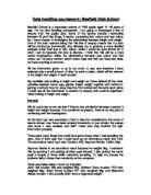
The sixty sample student in years 7 -11 showing their height (m) and weight (kg).
Now, you can see from the scatter diagram that there is definitely a clear relationship between height and weight and therefore, proves that my hypothesis (the taller the person is, the more they will weigh) is correct.
y = 38.57x – 11.074
This is to say that the gradient is 38.57 and -11.074 is the y intercept.
To find out the gradient you have to do this:
Δ y change in y y² - y¹
= =
Δ x change in x x² - x¹
You choose to points on the line of best fit on the graph; () and ().
Therefore you do :
y² - y¹ = () = =
x² - x¹ ()
Then to find out the y-intercept you insert a y and x value into the formulae, y=mx+c where mx= gradient and c= y intercept.
(?x,?y)
?y = 38.57 x ?x + c
?y = ? + c
?y – = c
c = - 11.074
Rearrange:
y = 38.67x - 11.074
Plot the line of best fit – how you got it
Talk about real life
Spearman’s Rank
R² = 1 - 6∑d
n³ - n
= 1 – 6x18127
60³ - 60
= 1 - 108762
215940
= 1 – 0.5036
= 0.4963
Round up = 0.5
By doing spearman’s rank you see whether the you have a positive/negative correlation and if you have a strong/weak correlation between two pieces of information. The nearer you get to 0 the weaker the correlation and the further away it is from 0 the stronger the correlation. if the number is negative hence there is a negative correlation, if the number is positive hence there is a positive correlation.
-1 0 1
My correlation was here (0.5), this is a positive correlation and is in the middle of 0 and 1 therefore there is a positive and medium correlation between height and weight.
Working out the standard deviation of the 60 students heights in years 7-11.
x = 97.16 x² = 158.22
x = Height (m) therefore x² = Height (m)²
∑= sum of
_____________
S.D. = √∑x² - ∑x²
n n²
_____________
= √ 158.22 - 97.16²
60 60²
__________________
= √ 158.22 - 9440.0656
60
3600
_________________
= √ 2.636987 - 2.62223936
________
=√0.014748
0.1214413 = Standard Deviation
0.014748 = Variance (The variance is just the standard deviation before you square route it)
Standard deviation is calculating weather your mean is accurate and good for a correlation. The nearer the standard deviation is to 0 the more good and reliable the mean is. Standard deviation works out how much either side of the mean can be accepted to be as the mean. For example say the mean was 5 and the standard deviation was 0.5 the mean can then be seen to be anything from 4.5 – 5.5. In my case my total mean of the samples is 1.63; meaning anything between 1.5085587 and 1.7514413 will numbers that will be covered.
Not only by working out the standard deviations you can see how good your mean is, you can also see if you have come across any anomalies.
Mean = 1.63 S.D= 0.1214413
1 S.D:
1.63 + 0.1214413 = 1.7514413
1.63 - 0.1214413 = 1.5085587
1.5085587 – 1.7514413
The number of students in the range (1.5085587 – 1.7514413) divided by the total amount of students (60) x by 100 = 72% of the students heights covered.
2 S.D:
1.63 + 2(0.1214413) = 1.8729 you do two lots of the standard deviation
1.63 - 2(0.1214413) = 1.3871 because you are working out 2 standard
deviations
1.8729 - 1.3871
The number of students in the range (1.8729 - 1.3871) divided by the total amount of students (60) x by 100 = 98 % of the students heights covered.
Working out the standard deviation of the 60 students weights in years 7-11.
x = 3083 x² = 163567
x = Weight (kg) therefore x² = Weight (kg)²
∑= sum of
_____________
S.D. = √∑x² - ∑x²
n n²
_____________
= √ 163567 - 3083²
60 60²
_______________
= √ 163567 - 9504889
60 3600
____________________
= √2726.116667 – 2640.246944
_________
=√85.869723
9.266591768 = Standard Deviation
85.869723 = Variance (The variance is just the standard deviation before you square route it)
Standard deviation is calculating weather your mean is accurate and good for a correlation. The nearer the standard deviation is to 0 the more good and reliable the mean is. Standard deviation works out how much either side of the mean can be accepted to be as the mean. For example say the mean was 5 and the standard deviation was 0.5 the mean can then be seen to be anything from 4.5 – 5.5. In my case my total mean of the samples is 52.08, meaning anything between 42.81340823 and 61.34659177 will numbers that will be covered.
Mean = 52.08 S.D= 9.266591768
1 S.D:
52.08 + 9.266591768 = 61.34659177
52.08 - 9.266591768= 42.81340823
42.81340823 - 61.34659177
The number of students in the range (42.81340823 - 61.3465917)) divided by the total amount of students (60) x by 100 = 77% of the students heights covered.
2 S.D:
52.08 + 2(9.266591768) = 70.61318
52.08 - 2(9.266591768) = 33.54682
33.54682 - 70.61318
The number of students in the range (33.54682 - 70.61318) divided by the total amount of students (60) x by 100 = 97% of the students heights covered.
My Second Hypothesis
I will then explore into the fact that boys in year 11 will be taller than the girls in year 11.
86 Females
84 Males
86
170 x 30 = 15.1764 – rounds to give you 15
84
170 x 30 = 14.8235 – rounds to give you 15
Therefore I am going to pick 15 Females from year 11 and 15 males from year 11. I will be doing this via selective sampling.
I chose to do selective sampling because, stratified sampling is used to fairly work out how many certain random samples from (e.g.) a year you take from a piece of data. In this case there is already an equal and fair amount for males and females (15 each), so a stratified sample isn’t necessarily needed.
Selective sampling is when you want to select a certain amount of % of a certain amount of something. E.g. 50% of 170 students in year 11.
1
5 = 20% i.e. 1 out of every 5 students is chosen.
First I have to find a random number between 1 and 5 i.e. 0.989654 x 5 = 4.94827
Rounddown to give the number 5.
I will give each female in year 11 a number and I will also give every boy in year 11 a number.
I will pick:
5,10,15,20,25,30,35,40,45,50,55,60,65,70,75.
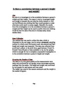
From looking at this graph you can see that there is a negative gradient of -0.1584 and also that the line of best fit will go through the point 1.4048 (y intercept, where the line is intercepted by the y axis).
Talk about real life
Spearman’s Rank
R² = 1 - 6∑d
n³ - n
= 1 – 6x426
30³ - 30
= 1 - 2556
26970
= 1 – 0.09477
= - 0.9
By doing spearman’s rank you see weather the you have a positive/negative correlation and if you have a strong/weak correlation between two pieces of information. The nearer you get to 0 the weaker the correlation and the further away it is from 0 the stronger the correlation. if the number is negative hence there is a negative correlation, if the number is positive hence there is a positive correlation.
-1 0 1
My correlation was here (-0.9), this is a negative correlation and is 0.1 off -1 therefore the is a negative and strong correlation between the height of females and males in year 11.
Stem and Leaf Diagram
Year Eleven - Females
KEY:13|7 = 1.37
Year Eleven - Males
KEY: 15|1 = 1.51
From this table there is a clear indication that males in year 11 have a higher height than females in year 11. Firstly the males mean is 1.662 m is taller than the girls mean of 1.624 m. Also the mode for males is 1.62 m whereas the mode for females is 1.63 m. The median for males is 1.65 m which is more than the female’s median which is 1.63 m. Finally, you can see that the range is higher for females this means that there are more students below 1.63 m (which is the median) than there are females who are over 1.63 m.
Cumulative Frequency
Year 11 - Females
Year 11 - Males
From looking at the cumulative frequency graph that showed the relationship between females and males height in year 11, I saw that firstly for the males:
Upper Quartile = 1.715 m
Medium = 1.635 m
Lower Quartile = 1.60 m
IQR = 0.115 m
Females:
Upper Quartile = 1.705 m
Medium = 1.615 m
Lower Quartile = 1.535 m
IQR = 0.17 m
From this I can see that the upper quartile for males (1.715 m) was higher than the upper quartile for females (1.705 m). This to say that as the upper quartile starts higher than the females one and 15 students from each gender is picked this means that there will be more taller students for males. I can also see that the lower quartile for males (1.60 m) was higher than the lower quartile for females (1.535 m). This to say that as the lower quartile starts higher than the females one and 15 students from each gender is picked this means that there will be more shorter students for females. The median for males is higher than the median for females this shows that because males have a higher median most of all the boys will be taller than the girls. Finally, as the inter quartile range for males is shorter than the IQR for females (taking into consideration that the upper quartile and lower quartile for males is both taller than the upper quartile and lower quartile for females), this means that male students will be taller than the female students in year 11.
Frequency Density
Year 11 - Females
Year 11 - Males
From comparing the two histogram graphs; the height of the females in year 11 and the height of the males in year 11, you can see that 0-1.60 m is a more popular range for females than males, but for males the range 1.60-1.70 m, is more popular than females. On the other hand 1.70-1.80 m is a more popular height range than it is for males. Then again males have a frequency of 2 for 1.80-1.85 m but females don’t have any heights in that range. In conclusion, I feel that it seems that more males are taller than females; hence, meaning that my prediction that males in year 11 are taller than females in year 11 is right.
My Third Hypothesis
I will then to further my investigation, look at that the older you are in school years the more you will weigh and the taller you will be.
I will use the same samples which I used in my first hypothesis.
Stem and Leaf Diagram
Firstly, this stem and leaf diagram will be comparing the heights of all the 60 students I have picked in randomly in my sample in years 7 -11.
Year Seven
KEY: 14|2 = 1.42
Year Eight
KEY: 15|2 = 1.52
Year Nine
KEY: 17|0 = 1.70
Year Ten
KEY: 16|2 = 1.62
Year Eleven
KEY: 15|8 = 1.58
Using the stem and leaf diagram I can work out this:
Total average mean = 1.63 m (1.51 + 1.62 + 1.64 + 1.67 + 1.71 m)
5 (number of years)
Total Mode = 1.55 m (the most popular height in my sample)
Total median = 1.65 m (1.73 m 1.68 m 1.65 m 1.57 m 1.52 m)
Total range = 0.56 m (1.86 - 1.30 m)
Middle Number
As you can see in the table above it clearly show that as the year (e.g. 7 - 11) goes up so does the height increase.
The mean in:
Year 7 - 1.51 m
Year 8 - 1.62 m
Year 9 - 1.64 m
Year 10 - 1.67 m
Year 11 - 1.71 m
Not only from this do you notice that as the year goes up so does the mean, you also can see from this that the difference between year 7 and year 8 is the biggest increase, from 1.51 m – 1.62 m which is a 1.1 m difference.
The mode in each year also increases; Year 7 - 1.45 m, Year 8 - 1.55 m and so on. (You can clearer see by looking at the table).
The median is also increasing in every year that goes up; it ranges from in year 7 – 1.52 m year 11 – 1.73 m.
Stem and Leaf Diagram
This stem and leaf diagram will be comparing the weights of all the 60 students I have picked in randomly in my sample in years 7 -11.
Year Seven
KEY: 2|6 = 26
Year Eight
KEY: 4|6 = 46
Year Nine
KEY: 5|9 = 59
Year Ten
KEY: 7|5 = 75
Year Eleven
KEY: 6|2 = 62
Using the stem and leaf diagram I can work out this:
Total average mean = 52.08 kg (43 + 51.3 + 52.8 + 57.3 + 56 kg)
5 (number of years)
Total Mode = 45, 49, 60 kg (the most popular weights in my sample)
Total median = 52 kg (57.5 kg 56 kg 52 kg 49 kg 45 kg)
Total range = 49 kg (75 – 26 kg)
Middle Number
The mean in:
Year 7 – 43 kg
Year 8 – 51.3 kg
Year 9 – 52.8 kg
Year 10 – 57.3 kg
Year 11 – 56 kg
From this you can notice that as the year goes up so does the mean. But in year 10 it has the highest mean, so when it comes to year 11 the mean drops only slightly to 56kg. This may seem to go against my hypothesis so I have found out that only some of my predictions are correct be to an extent about the older you are in school years the more you will weigh but the more you will weigh and the taller you will be has been clearly been shown above.
The mode in each year also increases; Year 7 – 45 kg, Year 8 – 49 kg and so on. (You can clearer see by looking at the table). Again, until year 10 where it goes up to the highest mode 60 kg it then decreases in year 11 where it drops as low as 48 and 56 kg. This also adds to the fact that only to an extent about the older you are in school years the more you will weigh.
The median is also increasing in every year that goes up; it ranges from in year 7 – 45 kg year 10 – 57.5 kg. Furthermore, in this case the medium for year 10 is higher than the year 11’s median of 56kg. This is also another factor which helps to prove that my hypothesis was wrong to an extent.
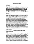
From the graph above there is a clear indication that overall the older you are in school years, the taller you are.
Again in the graph below there is an obvious view that the taller you are year of school most likely the taller you are going to be. This shows that my hypothesis is correct because I predicted that the older you are in school years the taller you will be.
From the graph above there isn’t really any indications of the relationship between years 7-11, whereas the graph below show that the height goes up as the year group goes up till year 11 where there is a decrease in weight. This shows that my hypothesis is wrong to extent because I predicted that the older you are in school years the more you will weigh, and quite clearly this is wrong to an extent.