On the following page a bar graph is shown to ensure the results are clear to understand:
Observations and conclusions:
- The bar chart above shows how the Year 11 group were closer on average to the 8.4cm length.
- The Year 7 group over estimated, whereas the Year 11 group under estimated.
- On average, there is a 1.17cm difference in the two sets of results. The Year 7 group were 0.88cm out from the genuine length. The Year 11 group were just 0.29cm away.
- The standard deviation results show that the Year 7 group had a much more spread out range of data compared to the Year 11’s. On average, the Year 7’s estimates were 3.0cm away from the mean average. As for the Year 11 group, they were just 1.56cm out from their mean average.
- From just looking at Year 7 and Year 11, I may not have got a conclusive in depth result. I have found out that, on average as you get older the mean average gets closer to the actual length of 8.4cm. Although this is on average, I can not always be sure that these results are reliable as the standard deviation for each year group are varied.
To conclude the comparison of Year 7 and 11 I can say that the Year 11 group came out on top. They had a far better mean average and standard deviation on average. Although the Year 7’s data wasn’t that reliable due to their standard deviation result I still would say that the age difference was what affected the results. 5 years difference is a huge amount when dealing with experience. The Year 11’s are at GCSE stage, therefore would have a much better perception of estimating then of the Year 7’s who have just began secondary school.
Conclusion on investigating the variable: Age
When looking simply at the basic tests I can see a pattern that shows that as you increase in age, the error of the average estimate decreases. This may be the case, but when I looked closer at many of the results I could see that the dispersion of data was quite large, therefore emphasising that the data is unreliable. The mean averages were all rounded to two decimal places and the closest year group to the actual length of 8.4cm was Year 11 with 8.11cm. When extending the investigation by looking at specific ages, the best age group were the 15 year olds with an average of 8.72cm. Although the oldest age group, the 16 year olds didn’t come out on top, they still only had a 0.62cm margin of error. This may have occurred due to a couple of outliers affecting the mean average.
Investigating Intelligence
I have now completed investigating age. I am now going to study intelligence to see whether this affects a person’s ability to estimate. Firstly I will look at each year groups higher sets, comparing the results and aiming to find a pattern. Following on from that I will analyse the lower sets from each year group, like I did earlier with the higher sets. To ensure I keep the investigation accurate, averages will be rounded to 2 decimal places as all my other results have. For each of the tests to do with intelligence, I will investigate the Mean average & Standard Deviation to see how reliable each set of results are.
Higher sets for each Year group
I’ll now show these results in a bar graph:
On the following page I’ve drawn on each of the higher set year group’s results in box and whisker diagrams to show the spread of data:
Observations and conclusions:
- When observing the results I firstly recognised that the year 7 higher set and the year 9 higher set both have the same mean average of 8.94cm. I then looked at the standard deviation to see how they compared and saw that the higher set Year 7’s data is more than twice the dispersion of the year 11’s.
- From the box and whisker diagrams I can see that the Year 7 group has the most spread out data. Also, the dispersion of data decreases as the ages progress.
Now I’m going to study the lower sets to see if any of the results are close to one another or far apart. From investigating all the lower set groups I wouldn’t expect any group to have a close mean average to 8.4cm. I think this due to their lack of mathematical ability and therefore not having a strong perception of estimating lengths.
I’ll now represent this data in a column chart to allow the reader ease of viewing:
Observations and conclusions:
- From studying the bar graph and results table I can note that the Year 8 and 11 group were the two closest averages to the 8.4cm length.
- The other three years, 7,9 and 10 all over estimated, especially Year 10 who on average estimated 9.76cm. An error of 1.36cm.
- By looking at the standard deviation results, I noticed how the Year 8 group’s results were very unreliable. There could have been many over and under estimated results which when averaged out made a reasonably close mean average.
- The most reliable data was the Year 11 lower set with a Stan.Dev of 1.63
From examining the investigation of ‘Lower set Year groups’ I can state that the Year 11 group results were the most accurate. This is because of their standard deviation being the lowest out of the five groups. Although the Year 8’s had the closest mean average, their standard deviation clearly shows that their results were not reliable. I’ve noticed on a few occasions that the age factor tends to affect a person’s ability to estimate and has done so in this investigation.
After having investigated both the Higher and Lower sets, I’m now going to compare each year groups sets to one another. By doing this I can see whether the higher sets are always better than the lower sets which you’d expect. I’ll use a variety of different graphs to show the results.
Comparing Higher and Lower sets for each Year group:
Here is a table of the results:
This line graphs purpose is to compare the Higher Sets to the Lower sets. From simply looking at the graph I can tell that the higher mean averages are to the right of the graph which is where the results of the lower sets are plotted. Towards the left, I can see how the line keeps decreasing as the year groups reach year 11.
Calculations
Observations and conclusions:
When comparing the Higher sets to the Lower sets I can conclude that for:
- Year 7: The higher set, on average estimated closer than the lower set by 0.68cm.
- Year 8: The lower set, on average estimated closer than the higher set by 0.83cm
- Year 9: The higher set, on average estimated closer than the lower set by 0.2cm
- Year 10: The higher set, on average estimated closer than the lower set by 1.38cm
- Year 11: The lower set, on average estimated closer than the lower set by 0.03cm
From simply looking at these results I can see that the Year 8 and 11 lower set groups estimated closer on average then their years higher set. In addition, Year groups 7,9 and 10’s higher sets estimated closer on average than their lower sets. Although you would first think that Higher sets won by 3 to 2, when you look at Year 8 there is very unreliable data which I would predict their higher set to do better than the lower set due to there standard deviation. I’ve studied how different each year group sets were from one another and the closest year group were the Year 11’s. The difference between their higher and lower sets mean average was just 0.03cm. This shows how their very similar and not much different in mathematical ability to estimate. To support this, the standard deviation results show that both Year 11 sets have a compact range of estimates. This proves their mean average is accurate.
Conclusion on investigating the variable: Intelligence
I’ve now analysed the investigations to do with intelligence fully and can conclude that when all the data are reliable and accurate, the higher sets in each year group would come out on top when compared with their year groups lower set. In my hypothesis I said that I felt experience in estimating would affect the results and I can say that this supports my prediction. Although the results show otherwise, many of the mean averages are unreliable due to their standard deviation, when taking this into account overall the intelligence of a person would affect a person’s ability to estimate. During the investigation where I compared each year groups higher and lower sets, only year 8 and 11 results showed the lower set doing better than their higher sets. For the year 8’s, the lower sets stan.dev was twice the amount of the higher sets. Finally, for year 11 the mean average was only different by 0.03cm and also their stan.dev weren’t very similar. In this case I would say the two sets were equally as good due to the lack of accuracy.
Investigating Gender
In this part of the investigation I will investigate Gender. This is to see whether being male or female means your ability in estimating is better. To begin with I’ll study male against female. Then I’ll go onto investigate different year groups with the sexes. For example I’ll look into whether being a female in year 11 means your estimating ability is better than a female in year 7. Like I’ve done in both of the other variables, age and intelligence, I will show the results in a range of different charts and graphs. This will allow the reader a better view of the results and data. As well as this I’ll be able to make observations from being able to see the data in different charts.
Comparing Male to Female
Gender has many different areas which can be covered. I’m starting off with simply comparing all the males to all the females:
From this table, I can see that all females are better at estimating then all males.
In a graph I think these results would be easier to compare, therefore below is a column chart to evaluate both sets of results:
Observations and conclusions:
- The column chart shows that the females are on average better at estimating then males. The males mean average was 9.16cm, compared to the females closer 8.57cm estimation average.
- In addition, the female’s standard deviation showed the data to be more compact than that of the Males. This supports the mean average results as the results are more reliable.
- I wasn’t surprise to see that both male and female on average had over estimated. When looking back on other tests, nearly all the averages show the groups to have over estimated.
As a conclusion, the female group have been shown to be the better at estimating. The male group neither had better mean average nor standard deviation. This emphasises how the Males results weren’t even completely accurate and still didn’t come off the better of the two sexes. From this investigation you would agree with saying that being a female affects your ability to estimate.
As a more in depth method of analysing Gender, I will investigate the results of comparing each different Year group sex. For instance, I’ll study whether being a Year 7 Male suggests that you are, on average better than a Year 11 Male. I hope to achieve some conclusive results and display them in a number of ways to show my findings.
On the following page is a table of results to do with the investigation described above:
Comparing Year group sexes
To enable the reader to view the results in a more clearer way I’ve presented the data in bar graph:
Observations and conclusions:
- The results table and the bar graph show to me that the year group sex with the lowest standard deviation is the Year 11 Males. Just 0.01 more than them were the Year 10 Females so they were two very close groups.
- However, when concluding the mean average calculations I can see that Year 10 Female were the closest, followed closely behind by Year 8 Female. The Year 10 Female recorded a mean average of 8.53cm, just 0.13cm off the actual length of 8.4cm.
- The group which over estimated by the most were the Year 7 Males. They, on average estimated 9.84cm, an error of 1.44cm.
- The group which under estimated the most were the Year 11 Females. They, on average under estimated 8.08cm, an error of 0.32cm.
I’m now going to represent the results I’ve calculated in a smooth line curve diagram: , from doing this I’ll be able to have a clearer idea of whereabouts the bulk of the data ranges from:
Observations and conclusions:
- The curve line chart above shows to me that Year 10 Females are the best out of the investigates groups.
- Furthermore, the chart shows peaks and lows where their have been high over estimates and under estimates.
- When looking at the distance between Year 7 male and Year 9 male, I can see that the curve goes up, then down and then finally back up.
- At several points during the graph, the curve is uneven and always changing direction. At the beginning, the line slumps considerably from around 9.8 to just above 8.6. This is a large amount considering the axis scale.
- From where Year 10 males is, to the last group Year 11 males, the curve drops from 9.6 to 8.1. This is the first time I’ve noticed the line reach below the mark of 8.4cm.
In conclusion to all my observations, I conclude that the curve line graph shows the sexes to record very different results to one another as you reach an older year group. The difference between the Year 7 sexes mean average was 1.19cm, compared to the Year 11’s 0.07cm difference. On the other hand, the year 7 sexes data was very spread out and unreliable compared to the Year 11’s very reliable and accurate results.
To extend the way in which I present the results, I’m now going to produce a skew diagram in which will show where the main bulk of the data is situated:
- See graph paper
Observations and conclusions
- The Male Skew graph shows that most of the data collected was either in groups (7.5 - <10) or (10 - <12.5).
- 75% of the male’s data was collected between these two groups.
- In stead of decreasing to the end, the Males graph shows that the skew increases when it reaches the group (15 - <17.5). From then on it decreases to 1 where it remains.
- When I look at the Females Skew graph, I can see that the group which had the largest number of estimates was (7.5 - <10). This group had 42% of the Females data.
- Both groups to the side of (7.5 - <10) were close to one another with (5 - <7.45) having 24% of the data and (10 - <12.5) with 27%.
- The one main comparison between the two sexes was that the females graph increased fully and then decreased gradually, whereas the Males increased twice at different stages.
The Males graph shows that it collected two large parts of the data in the groups (7.5 - <10) and (10 - <12.5). From this happening, there is less data which could have been recorded else where. This may have been the reason why the group (12.5 - <15) increased, whereas the pattern would have been to carry on decreasing. For the Females though, their graph followed the pattern perfectly by increasing gradually to their highest point which was a frequency density of 42 in group (7.5 - <10), then decreasing steadily until then end.
Calculations
Final Conclusion
Overall this investigation has proved to be a success. I have studied the three variables; Age, Intelligence and finally Gender to the best of my ability. The tests I have carried out have all been concluded thoroughly and written accurately. At each stage during the investigation I have looked out for any patterns emerging and have shown these in my Observation section.
I began this investigation with the aim of finding out whether either: Age, Gender or Intelligence affects a person’s ability to estimate.
I found that all three variables affected the results in different ways. To begin with I studied Age because it seemed that this would be the main factor in this investigation. In my hypothesis I predicted that Age would affect a person’s ability because of the lack of experience fro the Year 7 group compared to the Year 11. The results tended to agree with my hypothesis although from the Standard Deviation results, it seemed the results weren’t completely reliable. Therefore I am not able to state that Age has affected a person’s ability to estimate, but that on average the results do show that Age has affected a person’s ability to estimate.
By looking back on the observations taken from the results, I would say that when investigating Age I went into considerable depth to conclude whether there is an affect on a person’s estimation ability. I started by looking at all five year groups and then went on to compare the oldest year, year 11, to the youngest, year 7. Having analysed these, I went on to study the Age groups from age 11-16. This I felt would show a larger range of results but in fact wasn’t as concluding as expected. The results showed that age you increased in age you do get better at age. Nevertheless, the same problem has occurred in which the results can’t be completely reliable due to the Standard Deviation results showing unreliable data collecting.
In the part of the coursework, where I investigated Intelligence I expected for the Higher sets to come out on top of the Lower sets. This is because in my hypothesis I predicted that the more intelligent groups would do better as they had a better ability in mathematics then that of the lower sets. From analysing the results, they show how I was partly correct due to three higher sets out of the five were the better. In addition, the standard deviations show that the lower sets data was extremely unreliable. From this, I noticed that their was a good chance that if all the data had been reliable the higher sets most probably would have come out on top in all year groups. As a conclusion to investigating Intelligence I said that the mean average results showed the sets to be fairly the same. Although these were the results, the accuracy and reliability was uncertain from the standard deviation results.
In the final part of the coursework, I studied the variable Gender. I began off by comparing all the year groups for male to all of the females. The results showed that the Females were better overall. I then followed on by looking as a more in depth approach to each Year group sex. I found that the results seemed to follow the pattern by which as you got older the mean average became closer to the actual line. The only outlier as you may put it was the Year 10 Male’s which was well on average over estimated. This I found a surprise as a whole Year, they were a good class as a whole.
At a few points during the investigation I have looked at two variables. I have tended not to change them frequently to enable ease of viewing and clear understanding of my findings throughout the coursework.
In terms of accuracy, I feel this investigation has been a success. I have extended each variable and have recorded some conclusive results. Although I encountered a few problems I managed to overcome them and conclude that all three variables affect a person’s ability to estimate just in different quantities. For Age, I’d say that the variable affected the results the most. The experience factor I feel is very vital. For Intelligence I feel this affected the results a substantial amount due to the mathematical ability factor. Finally Gender, I don’t feel being either male or female affected the results but still gave some interesting readings to analyse and observe.
Page 18 – To explain the misunderstanding towards STAN DEV P
When I began this investigation I was under the impression that the Mean Average and Standard Deviation functions on Excel were the closest way in which to find the averages for each set of data. I used these functions to record results and produce charts and graphs to show the data clearer and on a larger scale. The three variable investigations: Age, Intelligence and Gender all have the results of Stan Dev. Recently though, my class have discovered that there is actually a function called Stan Dev P which records a more accurate range of data. The Stan Dev function I’d been using has been found to simply take an estimate made by Microsoft Excel. Therefore, I have calculated all the Stan Dev P results for the necessary groups which I have investigated to ensure the results are accurate and precise. Without doing this I wouldn’t be able to say I completed the investigation fairly and am confident of my concluding statements. Below is a table with the functions I’ll be recording:
- Mean average
- Standard deviation
- Standard Deviation P
In addition to these three, I will add a final fourth calculation to view the average error between the Stan Dev results to the more accurate Stan Dev P.
Now that I have shown the results for both Stan Dev and Stan Dev P, I can prove how the most difference to the results I have investigated is 0.09cm. This was the Year 7 Higher Set. Their previous Stan Dev was 3.24, compared to their Stan Dev P of 3.15. To conclude this problem I have encountered, I can say that the issue has been resolved and no results were vitally affected by the setback.