PLAN
Firstly, I will create a table that will only contain information relative to my investigation. Then I plan on selecting a random sample of cars from the selection so that there are a smaller number of cars for me to work with. This may make it easier for me but may also affect the accuracy of my results. I will go on to calculate the percentage depreciation for each of the 30 cars that I will have randomly chosen and put this information into a table.
Once I have done all of this I will start to test the factors that I think will affect the prices of used cars. I will test the make and colour on box plots, and the age, mileage and insurance group on scatter graphs. After analysing all of the graphs I will report my findings and give a conclusion and evaluation.
RANDOM SAMPLING
I have grouped the 25 makes of cars into 10 relevant groups that I may be able to carry out random sampling to a degree of accuracy. I plan to shorten the list of 100 cars to 30. I am carrying out the random sampling because it eliminates any biases on my behalf and it provides me with a smaller amount of data for me to work with and makes it easier for me to test the data, analyse it and obtain results.
Ford (16)
16/100 x 30 = 4.8
Vauxhall (13)
13/100 x 30 = 3.9
Nissan (6)
6/100 x 30 = 1.8
Renault and Peugeot (10)
10/100 x 30 = 3
Rover (12)
12/100 x 30 = 3.6
Fiat (10)
10/100 x 30 = 3
Volkswagen (7)
7/100 x 30 = 2.1
Mercedes, BMW, Audi, Land rover. (7)
7/100 x 30 = 2.1
Luxury Cars [Porsche, Lexus, Bentley, Rolls Royce] (4)
4/100 x 30 = 1.2
Other (15)
15/100 x 30 = 4.5
PRICE DEPRICIATION
I will plot all of my graphs against price depreciation. This is because I cannot plot them against current price, as this will cause many anomalous results considering that there are some expensive cars that are only one year old whereas there are some cheap cars that are very old. However, the only graph that I plotted against current price was the insurance group because the insurance group has to do with expensive cars and cheap cars. I will use the following formula to find the price depreciation.
(Difference*/Original price) x 100 = % depreciation
* original price – current price.
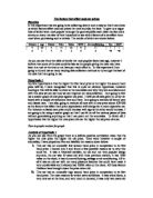
Age against Price depreciation
ANALYSIS
This graph illustrates a moderate positive correlation, which means that the older a car is, the more it has depreciated making it cheaper. The correlation isn’t strong possibly due to the use of a small sample of subjects and as I then generalized to the whole population from this sample. A sample size of 30 cars isn’t enough to generalize from in this case. Also, the cars were not all of the same make which means that they were from different price ranges causing anomalous results. However, the correlation is strong enough to prove my hypothesis correct.
From the graph it can be seen that there are more cars that are 6 years old than any other age. However, it can be noted that they all have different price depreciation. This is not to say that the age doesn’t affect the price depreciation, but shows that there are other factors that affect the price depreciation.
Mileage against Price depreciation
Analysis
This graph shows a moderate positive correlation showing that the higher the mileage on a car the more it has depreciated. The correlation isn’t strong, as accuracy may have been lost due to small sample size and also, the car from the expensive bands as well as the cars from the cheaper bands cause many anomalous results. The correlation is sufficient to deduce that the mileage does affect the price of second hand cars.
It must be taken into consideration that the graphs only show one of the factors while there are other factors that could be interlinked with the one factor shown and therefore show discrepancies or inaccurate results.
Most of the data is centred around the 5000km mark showing that most of these cars have a price depreciation of 70-80%.
Insurance group against second hand price
Analysis
Firstly it must be noted that this graph has been plotted against 2nd hand price and not price depreciation, as it was not possible to plot the insurance group against the price depreciation. This graph shows little or no correlation. There are anomalous results due to the factors that I have mentioned in the other graphs. Usually the insurance group should affect the second hand price but I think that the result I have obtained is due to loss of accuracy and discrepancies.
Most of the cars are underneath the £10000 boundary but the spread is quite far ranging from group 1 to group 16. This just shows that it isn’t only the price that determines the insurance group of a car, but also factors such as its top speed, how old the driver is, how well maintained it is, the amount of people being insured on the car etc.
Conclusion and Evaluation
In conclusion, three of the five factors that I chose turned out to be correct while two turned out to be incorrect according to the results obtained in this investigation. The correct ones were the make, age and mileage while the insurance group and colour were incorrect.
It must be taken into consideration that all the factors are interlinked and therefore could have caused anomalous results or discrepancies.
None of the graphs showed strong correlations showing that there are many factors that affect the price depreciation and they are all interlinked and are made obvious on the graphs.
I could possibly have obtained better results if I had tested more, or even all the cars. This would give me accurate results but would be time consuming. Also, on the box plots I should have used a wider variety/range of cars to show me the contrasts and my results better.
As there are so many factors that do affect the prices of used cars, in future experiments I could investigate using more factors such as the price when new and the amount of owners the cars had.
I could have extended my investigation by using standard deviation to estimate the spread of my data before plotting the graphs. This would have given me an idea on whether my predictions were valid or not.