Because the damping is due to the resistance in the liquid, the damped term is the resistance. In my assumption I said that the resistance was proportional to velocity. So. In this case velocity is , hence . My first model of this situation is completed. The model is as follows:
I am going to solve this differential equation. This is a second order differential equation. Following is the steps I have taken to solve this second order differential equation.
Aux. equation
Case 1:
General solution
It can be written as
It is an overdamping.
Case 2:
General solution
It is a critical damping.
Case 3:
General solution
It can be written as
This is an underdamping.
In the differential equation there are two parameters which are and . I would like to make a prediction on those values of the parameters. As simple pendulum motion is an approximate SHM, the time period is constant. We are able to find out the value of . The diagram below shows a simple pendulum motion.
The acceleration in the transverse direction is given by.
Applying Newton’s second law in the transverse direction gives
.
Dividing both sides by m and using the small angle approximation, the equation of motion is
.
This can alternatively be written as
or
In this case because is the only factor which can vary x which is the displacement from centre to the current pendulum bob location (length of the string is constant). Hence I can replace by x. The equation will looks like this: or . From this equation, we know that . In this particular coursework the length of the string I use is 1 meter long, hence where g is 9.8.
The damped term in fact is the resistance. I did a separate experiment in order to find the resistance.
What I did is that dropped the pendulum bob into a long tube full of water from the surface of water. I made a mark on the tube whose position is 0.2 meter from the surface of water. I would like to record the time which the ball took to cover this distance. In this experiment I assumed that the acceleration in this period is constant and the ball did not reach its terminal velocity in the 0.2 meter distance. The left hand side diagram shows the set of the experiment.
In order to reduce the error, I just took the reading from the first 0.2 meter and I repeated this experiment twice. According to Chaos theorem, in any numerical estimation the small error at the beginning will produce a very big difference at the end. If I made the second mark is 0.2 meter lower than the first one and took the reading, all my basic data for calculation (i.e. initial velocity) is estimation from my first approximation. As I taking more estimation, the error will be too big to make the results of this experiment unacceptable. Also I cannot do the experiment only once to get the results. Therefore I repeated the experiment twice rather than taking three readings from one experiment. The following table shows the results I have obtained.
Since I would like to find the parameter between resistance of motion and velocity, I should take out the buoyancy effect during my calculation. I put this ball into a glass which is full of water, and I put this glass inside a bowl. When the ball dropped into the glass, some water overflowed to the bowl. I measured the weight of the overflowed water (first measured the weight of the bowl and then took the reading of the bowl with water, finally minus the weight of the bowl from the total weight.) that is the buoyancy act on the ball when the ball is in the water. I buoyancy is about 3N (in fact it is 2.958N).
We have the equation . I have already known s which is 0.2 meter, t which is in average 0.37 second and u (the initial velocity). Because I released the ball from the surface of the water, the initial velocity is 0.
=〉
∵F=ma where F is the resultant force
∴
The average speed is the total distance divide by the time taken. . Therefore the radio of the resistance and speed change is about 7.1743. I gained an equation .
The completed differential equation is as followed:
By solving this equation, I obtained the Aux. Equ. is . Therefore and . The general solution of this differential equation is .
I wish to set the start angle is 17 degree. Sin170 is about 0.3. Therefore initially x is 0.3 meter. And initially the speed is 0 as well. Then I get the initial situation.
When and .
Differentiate the general solution:
Substitution these data in the general solution, I obtained two equations
The particular solution is
According to this graph, since t cannot be negative, the smallest value of t whose corresponding values of x can be approximate 0 is 3.75. ( when )
When t is 0.37, x is approximate 0.2; when t is 0.8, x is approximate 0.1.
From this equation I could make a prediction of the damped oscillation experiment. According to the particular solution I obtained, I have to say it is an overdamping which means the system will not oscillate! As the resistant force is too big the pendulum bob will stop at the centre. It will not do the simple pendulum motion. The ball will stop about 3.75s after it be released.
- Conducting the experiment
Here is the list of the equipment I used in the experiment.
- pendulum bob
- string
- stand
- stopwatch
- container
- ruler
- plastic card (with distance marks)
The diagram below shows the set of the experiment.
The distance from the pendulum bob to the centre line (the dot line in the diagram) is 0.3 meter. As I assumed that it is a SHM, the distance which be covered by the bob is 0.3 meter. I used a pair of chopsticks to release the bob. The reason why I did this is chopsticks will produce weaker wave when it is moving than the wave produced by my hand. I have already assumed that there is no side force. Therefore the stronger wave will make the bigger error. I also marked the centre line on the back of the container. I watched the motion from the front of the container. Because I assumed that the string is always straight, when the string and the mark are at superposition, the pendulum bob is at the centre.
The plastic card looks like the following diagram.
It is used to measure the time when x=0.1 and x=0.2.
I did this experiment five times and all the results are overdamping. I was not able to observe any oscillation at all. But the oscillation could be too small to be seen by human eyes. Hence I used a magnifying glass to help me to do the observation. Even using the magnifying glass to help the observation, I did not see any oscillation either. I recorded the time that the bob took to stop.
The average time is 3.82 seconds. The time matches the prediction quite well.
I also recorded the time which the bob took to cover the first 0.1m as well as the time which the bob took to cover the second 0.1m. The data is shown in the table below.
The average time of x=0.1 is 0.838s and the time of x=0.2 is 0.398s. These two points can roughly describe the sharp of the graph of the experimental results.
The result of the experiment strongly supports the theoretical prediction. It is overdamping and the pendulum bob stopped 3.82s after it had been released.
There are several errors be introduced into the experiment through the measurements. The biggest variability is the time. Because the time is quite short, my reaction time could influence the finally reading very much. Since I stay in the air and the motion was happening in the water, the refraction is another factor which could produce some errors. There are several other factors which will make some small errors for example the length of the string might not be exactly 1 meter and my assumptions as well.
- Comparison between the experimental results and the predictions
As I said in the previous part, my experimental results strongly support my prediction. The type of damping is the same, which is overdamping. The difference of the time that the ball took to stop is only 0.07 second. It could be due to my reaction time and the variability in the experiment. In fact the difference is very small.
Furthermore the graph of the equation I obtained is a particular graph of overdamping.
The dot line is the theoretical curve; the normal line the experimental curve. From the graph, we are able to see that the shapes of curve are nearly the same. This means the experimental results are very similar to my prediction.
I should say that the experimental results are perfectly matching the theoretical prediction.
Before I modelled the situation and did the experiment, I had made several assumptions. As far as I considering, the experiment is very simple, and the values of the data are pretty small, hence the assumptions in fact made less difference than the difference which was made by the variability in the measurements taken (especially my reaction time).
The only thing I am not sure is that whether it was an overdamped case or a critical damped case. Actually my theoretical prediction is based on the separate experiment. My reaction time should make all the values of time measurements bigger than it should be. The error bounds could be about 0.15 second. However if the time was a little shorter, my theoretical prediction might suggest that it should be a critical damping. Furthermore critical damping is not obvious in a physical situation. It can be very similar to the overdamped case. So it was possible for me to confuse two cases in the experiment.
Anyhow in the experiment I did, my model worked. It can represent the motion pretty well. Therefore I consider that this differential equation is the model of this situation.
- Assessment of the improvement
Since my reaction time is the biggest factor which effect on the experiment, I could use some better equipment to record the time for me. The reading will be more accurate than that I gained.
Also I can consider more factors rather than make assumptions. The model should be able to represent the real situation better.
Through this coursework I have obtained the differential equation which models the motion of a 1kg bob with 1 meter string in the water. The differential equation is . The general solution of the differential equation is and the particular solution is . The whole is system is overdamping.
The biggest variability in my coursework is the time measurements. It may change the parameter of the damped term. Therefore the type of damping may be changed as well. However according to the experiment, the whole system seems cannot be underdamping.
1. Differential Equations by Mike Jones and Roger Porkess