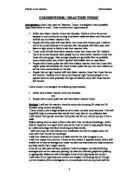
I will then drop the ruler without any notification and let the subject catch the ruler with their thumb and forefinger.
I will then measure and record in a table how far the ruler dropped in cm.
I will then repeat this a further 2 times so as to obtain 3 separate results which will enable me to take an average and make my data more accurate and help overcome any bias results that I might receive.
Once all my raw data has been collected I will investigate my data by finding averages such as the mean and plotting my data into relevant graphs and placing in appropriate tables and will investigate to see if my hypotheses are correct.
I will state if my hypotheses are correct and explain my findings found through out the duration of the investigation in my conclusion and sum up how well the investigation was carried out and how I may have improved it if I did it again in my evaluation.
Raw Data: I have recorded the pulse rate, gender and the results of each subject catching the ruler in the chart below. I have also calculated the mean average of the length the ruler dropped for each subject so as to make the results more accurate.
M
66
11
13
6
10
M
76
14
11
8
11
M
80
18
26
19
21
M
76
12
16
19
157
M
68
22
20
16
19.3
M
76
17
21
17
18.3
M
72
18
16
15
16.3
M
78
23
12
19
18
Results: Firstly, I will put the data collected into a scatter diagram to see if there is any possible links between gender, pulse rates and how they affect reaction times. This may also tell me whom generally has better reaction times and pulse rates.
The correlation of the plotted results of females on the scatter graph is positive. This suggests that the higher a females pulse rate is the longer it takes them to catch the ruler so a slower reaction time. Therefore implying my hypotheses those with lower pulse rates will have better reaction times to be correct.
There is positive correlation on the males scatter graph also. Like the females it inclines at about the same rate. However due to the males generally having a lower pulse rate it is positioned a little lower than that of the females. This strongly implies that the lower the pulse rate the faster your reaction time is and the males have better reaction times because they generally have lower pulse rates. From these graphs it is evident that males have better reaction times than females so suggesting both my hypotheses that males will have a better reaction time than females and that people with lower pulse rates will have better reaction times to be correct.
To investigate further I will draw a cumulative frequency table to enable me to put my data into a cumulative frequency curve. This will give me an approximate idea of what the median and the inter-quartile range will be. The table can also tell me how often a particular group of results was obtained.
Cumulative Frequency table to show mean average of female drops
Cumulative Frequency table to show mean average of male drops
I will now put the results from the cumulative frequency table into a cumulative frequency curve for males and females.
From both cumulative frequency curves I can take an approximate median and inter-quartile range for both females and males. It tells me that the females have a smaller and lower inter-quartile range, of 4 (16 – 12=4) than the males whom have a wider and higher one of 7 (19 – 12= 7). This suggests that the male results in general were more varied than those of the females. It also suggests that the approximate median average for females was 14. Whereas the approximate median for males is 15.5, which implies that the females have a lower reaction time on median average than males. However, there is only a slight difference.
To show the inter-quartile ranges and the median more clearly I have put the information from the cumulative frequency graph into a box plot for each of males and females.
These box plots define the varied results of the males and the closeness between the female’s results.
I will now use histograms to show the continuous grouped data.
.
3 ÷ 4= 0.7
24 ≤ d < 28
4
1
1 ÷ 4= 0.25
Drop (d) in cm
Frequency width
Frequency
Frequency Density
5 ≤ d < 8
3
0
0
8 ≤ d < 12
4
5
5 ÷ 4 =1.25
12 ≤ d < 16
4
6
6 ÷ 4= 1.5
16 ≤ d < 20
4
5
5 ÷ 4= 1.25
20 ≤ d < 24
4
4
4 ÷ 4= 1
24 ≤ d < 28
4
0
0
The standard deviation measures the spread of the data about the mean value. It can allow me to compare males and females, which may have the same mean but a different range.
Gender
Mean average
Step 1-2
Step 3-6
F
12
12- 13.9= -1.9
-1.9 x –1.9= 3.61
F
12.3
12.3- 13.9= -1.6
-1.6 x –1.6= 2.56
F
11.7
11.7- 13.9=-2.2
-2.2 x –2.2= 4.84
F
12.3
12.3- 13.9= -1.6
-1.6 x –1.6= 2.56
F
11.7
11.7- 13.9= -2.2
-2.2 x –2.2= 4.84
F
11.3
11.3-13.9= -2.6
-2.6 x –2.6= 6.76
F
7.6
7.6-13.9= -6.3
-6.3 x –6.3= 39.7
F
7.3
7.3- 13.9= -6.6
-6.6 x –6.6= 43.6
F
17.7
17.7- 13.9= 3.8
3.8 x 3.8= 14.4
F
13.3
13.3- 13.9= -0.6
-0.6 x –0.6= 0.36
F
20
20-13.9= 6.1
6.1 x 6.1= 37.2
F
253
243- 13.9= 11.4
11.4 x 11.4= 130
F
14
1413.9= 0.1
0.1 x 0.1= 0.01
F
22.7
22.7-13.9= 8.8
8.8 x 8.8= 77.4
F
20.3
20.3-13.9= 6.4
6.4 x 6.4= 41
F
13.7
13.7- 13.9= -0.2
-0.2 x –0.2= 0.04
F
15.7
157-13.9= 1.8
From the results of the standard deviation I can distinguish that the distribution round the mean average of the female and male frequency was very low. The standard deviation suggests that the female’s results are generally more spread out round the mean rather than the males whom are not so spread out. This means that males generally have similar reaction times rather than females whom the results imply to have more varied results.
Conclusion: From the data I collected I have found that males appear to have better reaction times than females, which seems to be linked closely to them having lower pulse rates. This suggests both my hypotheses to be correct and closely linked to one another. Although, on median average females have been implied to have a lower reaction time. However, the male and female median average are extremely similar so due to the males having a increasingly better mean average seem to generally have better pulse rates and reaction times. This proves that everyone has different reaction times, which can be altered by many different variables such as that as pulse rate.
Evaluation: I could have tested reaction times in a many more ways and did not have to use just light as a stimuli for the reaction time. I could have used sound like the reaction time for someone to hear the sound of a gun at a beginning of a race and to react to that and start running. Also the subjects results could have been affected by anything from light and sound distractions to whether they had consumed a substance containing caffeine before they had taken part in the activity set for them. Some of these will not have been able to improve on but others such as where and when I had collected my data may have made possible for bias results to come up in my investigation. Whether the subjects were tired, focussed, motivated will have made a difference to their performance as well so external influences can play a big part in the alteration of results. Also if the participant had carried out this particular type of investigation before or if they trained specially to improve a reaction like those whom train for sprinting would have had a clear advantage than those whom had not carried out the experiment before.
In my experiment I also found that an exact recording of how far the ruler actually dropped before it was caught hard and can be seen to have been rounded to the nearest centimetre, which will not have not given me very accurate results.