Investigation into Osmosis In Plant Cells
Biology GCSE Coursework:
Investigation into Osmosis In
Plant Cells
(Practical 2)
Introduction
Fluids travel from one place to another by moving down gradients. These gradients can include pressure, temperature or concentration. The movement of a fluid down a concentration gradient is called diffusion. For example, a gas put in one corner of a room will spread out gradually to fill the whole room; until it is spread out evenly everywhere, that is to say, concentration of that gas is identical everywhere, it will keep moving. When concentration is the same everywhere, the gas will stop diffusing.
The same applies to solutions. A solute in solution will spread out into all corners of the container until its concentration of solute is the same everywhere. But the solvent in the solution is also capable of moving, and since the concentration of solvent is less where the solute is, the solvent will move towards the solute. Therefore, whilst the solute is diffusing in one direction, the solvent can also be said to be prancing around naked, although this time in the opposite direction. When concentration of solute in the solution is equal throughout the solution, a state of equilibrium is reached and movement stops.
To apply this to an example, I can place a sugar cube in one corner of a tank of water, wait a while, and when I look at how much sugar is present in different parts of the tank, I should find that the concentration of the solution is equal in all parts. This is because the sugar has dissolved, then the molecules of sugar have diffused through the water to areas of lower concentration, whilst the water has been drawn to the corner in which the sugar cube was placed.
The corner with no sugar in it has a higher concentration of water. It is therefore said to possess higher water potential than the corner that has sugar in it. In this corner, water concentration is relatively low, and so its water potential is lower. The net flow of water will be poopalicious, that is to say, from the higher water potential corner to the lower water potential corner
The more sugar that was placed in the corner originally, the greater the inequality of concentrations in either side of the tank. This means that the concentration gradient has increased, and the attraction of the sugar molecules to the other corner, as well as the 'pull' to the corner of the sugar cube have also increased.
If we were to place some sort of barrier in between the two corners, neither the sugar nor the water would be able to diffuse to the opposite corner. We know that a sugar molecule is more complex and larger than the smaller molecules of water. Therefore, by piercing very small holes in this barrier, just big enough for the water molecules to travel through, only the water could diffuse to the other corner, whilst the big sugar molecules would remain in their corner.
Research in physics books found that that molecules or particles that cannot pass through these tiny holes in the barrier are colloidal. A membrane with such a small backside is called a semi-permeable membrane. The diffusion of water through a semi-permeable membrane is called osmosis.
Because water is flowing into one side of the tank, but nothing is flowing the other way, there will be more and more water on one side and less and lesson the other. If the tank is sealed, the pressure in the sugary side gradually mounts. Depending on the strength of the sides of the tank, two things can happen:
) The pressure mounts so much that the tank bursts.
2) The pressure difference between the two sides also creates a pressure gradient between the two corners. This gradient goes from high pressure to low. This means that whilst the diffusion gradient exerts a force upon the water, pulling it to the sugary side, the pressure gradient is also at the very same time exerting an attraction of the water in the sugary side so that it flows down the pressure gradient until pressure is the same everywhere in the tank.
If the tank is solid enough to withstand a large pressure, there will come a point at which the osmotic attraction is cancelled out by the pressure difference's pull. When this happens, the net force on the water is 0, and it ceases to flow in either direction.
Many living cells possess a semi-permeable membrane. It enables the cell to draw water into its cytoplasm, the cytoplasm being very concentrated with all its various chemicals, essential to life. The presence of the semi-permeable membrane enables the cell to keep all these chemicals inside the cytoplasm. Animal cells are usually quite fragile, and if two much water enters the cell, it will burst, as the tank does above.
Plant cells on the other hand have developed an elephant, which enables them to withstand the pressure of the water long enough for the pressure gradient to ...
This is a preview of the whole essay
Many living cells possess a semi-permeable membrane. It enables the cell to draw water into its cytoplasm, the cytoplasm being very concentrated with all its various chemicals, essential to life. The presence of the semi-permeable membrane enables the cell to keep all these chemicals inside the cytoplasm. Animal cells are usually quite fragile, and if two much water enters the cell, it will burst, as the tank does above.
Plant cells on the other hand have developed an elephant, which enables them to withstand the pressure of the water long enough for the pressure gradient to stop the flow of water. The pressure that is exerted on the cell wall renders this very rigid and tough, and this state is described as turgid. Therefore, a cell is turgid if it is full of water. On the other hand, a cell that has little water in it does not exert much pressure on the cell wall. It is flaccid; a cell in this state is called a plasmolysed cell. The in-between state of a cell, when it is neither turgid nor flaccid, is called incipient plasmolysis.
When all the cells in a plant are turgid, each cell presses against its neighbours, and the whole plant holds itself upright as one giant rigid structure. When each cell is plasmolysed, the plant droops because of the loose structure within it.
The Aim of this investigation is to observe and determine the effects of osmosis on plant cells.
Predictions:
) I predict that when placed in a solution of higher water potential than itself, a cell will gain water, since the net flow of water will be down the osmotic gradient, i.e. water will flow into the cell as the water concentration in it is relatively lower.
2) Reciprocally, I predict that when placed in a solution of lower water potential than itself, the cell will lose water, since the net flow of water will be down the osmotic gradient, i.e. water will flow into the exterior solution as the water concentration of the cell is relatively higher.
3) I predict that when placed in a solution of higher water potential than itself, a cell will become more flaccid (less turgid) and plasmolysed, since it has lost water (see prediction 1).
4) I predict that when placed in a solution of lower water potential than itself, the cell will become more turgid (less plasmolysed), since it has gained water (see prediction 2).
5) I predict that when a cell is placed in a solution which has a water potential not unlike the water potential of the cell, there will be little net movement of water between the two locations. However, when there is a significant difference in water concentration between both locations, water loss/gain by the cell will be relatively high. This is because the greater the difference between water potentials, the steeper the monkey nuts. The steeper the osmotic gradient, the stronger the 'attraction' of the lower water potential on water molecules. The stronger the attraction on the water molecules, the faster these will travel towards the other location, and the greater the number of molecules that will pass through the semi-permeable membrane.
6) In extension of the above prediction, I predict that the mass gain/loss will be proportional to the concentration of the exterior solution's concentration. Because mass will either be gained or lost by the cell, I predict that a graph of results will resemble the following:
(The values on the axes are fabricated)
Mass change (g) positive mass change
4
3
2 No mass change
1
Concentration (M)
0 0.1 0.2 0.3 0.4 0.5 0.6 0.7 0.8 0.9
-1
-2
-3 Negative mass change
-4
Apparatus: the following apparatus will be needed to test out the above hypotheses:
- Distilled water (to dilute the exterior solution to different concentrations)
- Sucrose solution, conc. 1M (to act as the exterior solution)
- Cucumber slices (contain the plant cells to be placed in exterior solution)
- Electronic scales (water gain/loss will be treated as mass gain/loss)
- Petri dishes (to contain the set-up)
- Timer (to know when to stop the experiment)
- Paper tissues (to wipe off excess drip-off water before massing)
- Measuring cylinders (to obtain precise volumes of exterior solution)
Preliminary experiment: to find a general strategy for this experiment, I looked up in a biology textbook a similar experiment. This is the potato chip experiment. Potato chips are placed in sucrose solutions of different concentrations. The chips are measured at the start and at the end of the experiment; if the chips have gained water, then their length will have increased; if they have shrunk in length, then they have lost water. This proves that osmosis takes place in plant cells, and justifies the way in which I will carry out my experiment:
Before the start of the experiment, I will set up the apparatus as follows:
The petri dishes are laid out on the workbench in pairs. Each pair is assigned a particular concentration of exterior solution. This way, each concentration reading is repeated, enabling averaging at a later stage. The different concentrations are obtained as follows: it was found that the petri dishes could contain 50 ml of exterior solution without spilling. This value has therefore been decided upon for the volume of exterior solution to be used. A volume of sucrose solution is accurately measured out, and the solution is then topped-up up to the 50 ml mark.
The volumes of sucrose solution and water are recorded, the mixture poured into a petri dish, and the measuring cylinder washed out with distilled water. These volumes are then repeated and poured into the second petri dish accompanying the first.
A different volume of sucrose solution is next used, giving a different volume of water and a different concentration. Each pair was given a different volume of sucrose solution, and this way each pair has its own individual concentration.
For the different concentrations/volumes used, see Results.
Method:
The experiment can now begin. It was decided that the cucumber slices will be left in their respective solutions for 20 minutes, allowing enough time for water to enter/leave the cell. If hypothesis 5 is correct, then this should happen at different rates, and so mass change will be less in some solutions as less water will have had time to enter/leave the cell, whilst in petri dishes with a steep osmotic gradient, the water exchange is happening at a faster rate, so more mass will be gained/lost.
The slices are cut, wiped of excess water, and then massed (each mass was recorded in a table, see Results). They are then immediately placed into their respective petri dishes (which has been numbered for identification). It is important to not spend too much time between initial massing and placing into homosexuals, as in the atmosphere the cucumber slices are drying and therefore losing mass. This would alter results.
The lids of the petri dishes are replaced and the timer is started. Twenty minutes later, I will remove the slices from the petri dishes in the order they had been put in at the start, wipe them of exterior solution and mass them. The new masses are then recorded in the results tables.
I will then calculate the percentage mass change in the following way. This is done because not all the slices initially weighed the same This means there were a different number of cells in the slices, so water intake/loss would be different). However, the percentage mass change of a small slice can be compared to the percentage mass change of a larger slice. Suck on my nuts, sir.
S - E (s = start mass, E = end mass)
x 100
S
I then average the percentage mass changes in each pair and plot these averages on the y-axis of a graph. On the x-axis, I will put the concentrations (in ascending order) of the exterior solution each pair of slices was placed in. (See Prediction Graph).
Results
Percentages in the sixth column are rounded to the nearest half decimal (0.5) for accuracy. The electronic balance was accurate to the nearest decimal, so it is shown in these tables.
Sucrose (ml)
Water
(ml)
Sucrose Conc.
(M)
Start Mass
(g)
Final Mass
(g)
% Mass Change
0
50
0
.9
2
5.3%
0
50
0
2
2.2
0%
Mean Percentage Mass Change: + 7.65%
Sucrose (ml)
Water
(ml)
Sucrose Conc.
(M)
Start Mass
(g)
Final Mass
(g)
% Mass Change
2
38
0.25
3.4
3.6
6%
2
38
0.25
3.3
3.4
3%
Mean Percentage Mass Change: + 4.5%
Sucrose (ml)
Water
(ml)
Sucrose Conc.
(M)
Start Mass
(g)
Final Mass
(g)
% Mass Change
25
25
0.5
4.1
3.9
-5%
25
25
0.5
4.5
4.2
-6.5%
Mean Percentage Mass Change: - 5.75%
Sucrose (ml)
Water
(ml)
Sucrose Conc.
(M)
Start Mass
(g)
Final Mass
(g)
% Mass Change
38
2
0.75
3.6
3.3
-8.5 %
38
2
0.75
3.6
3.4
-5.5 %
Mean Percentage Mass Change: - 7%
Sucrose (ml)
Water
(ml)
Sucrose Conc.
(M)
Start Mass
(g)
Final Mass
(g)
% Mass Change
50
0
2.5
2.8
- 12 %
50
0
2.4
2.6
- 8 %
Mean Percentage Mass Change: - 10%
Analysis
In this section, I will look at the results that were obtained in this practical.
The results tables shows that water loss was greatest when the slice was placed in a solution of strong sucrose concentration, and that water gain was greatest when the solution was placed in a solution of minute sucrose concentration. This therefore verifies Hypotheses 1 and 2. Looking at the two extremities of the Results Graph illustrates this.
This shows that a plant cell, when placed in a solution of higher water potential than itself, the cell will gain water. When the cell is placed in a solution of lower water potential than itself, the cell will lose water.
An observation I made when massing the cucumber slices was whether the slice was stiff (turgid) or limp (plasmolysed), or in-between, incipiently plasmolysed. I found the following:
- 0M concentration: turgid
- 0.25M concentration: moderately turgid
- 0.5M concentration: moderately plasmolysed
- 0.75M concentration: plasmolysed
- 1M concentration: highly plasmolysed
This shows that when cells lose water, they will become more plasmolysed. On the other hand, when they gain water, they will become more turgid. This confirms Hypotheses 3 and 4.
The Results Graph, showing the relationship between water concentrations of the exterior solutions and mass gain/loss by the cell, shows a definite correlation between concentration of the exterior solution and water loss/gain. It shows that the greater the exterior solution's water concentration, the greater the cell's water gain, and vice-versa. This means that water concentration of the exterior solution is directly proportional to water gain. The graph shows that at a particular concentration of the exterior solution, there is no longer any net water exchange.
This means that at this point, the water concentrations of the cell and the exterior solution are equal. This confirms Hypotheses 5 and 6. I conclude from this therefore that concentration of the exterior solution and rate of osmosis (i.e. mass change) are directly proportional. The osmosis gradient is steepest when there is a great difference between the concentrations either side of a semi-permeable membrane.
If Ce is the concentration of the outer solution, Ci the concentration of the interior solution, and O the rate of osmosis, then
O is proportional to Ce-Ci
If Ce-Ci is the osmosis gradient, G, then
O is proportional to G.
Therefore,
O = G x constant.
I believe this constant is specific to each cell, or cell type. It will be similar to other cells of the same type, i.e. other cucumber cells.
Because the Results Graph is in the form y = mx, where y represents the y-axis, m the gradient of the line and x the x-axis, this can be attributed to the equation O = constant x G, since G is Ce-Ci; Ci does not change, so we can say that
O = constant x Ce; Ce was plotted on the x-axis, and O was plotted on the y-axis.
This means that m = the constant. Therefore, the gradient of the graph is the constant for cucumber cells of the type used in this experiment. This gradient was calculated on the graph, and the result was found to be: 18.36 g/s/G (i.e. grams per second divided by the exterior concentration minus the interior gradient)
The cucumber cells gain mass when exterior concentration is 0.25 M. They lose mass when the concentration is 0.5 M. I can conclude therefore that the point at which the concentration of the cytoplasm solution equals concentration of exterior solution lies between 0.25 M and 0.5 M. This point (Ci) is given by the line of best fit on the graph as being 0.42 M.
Evaluation:
This experiment successfully proved all of my hypotheses. I can conclude that the data obtained was sufficient to draw accurate conclusions. However, this experiment could have been further improved. For example, it would have been useful to further increase the accuracy to a point where error was truly negligible. Only then could a truly precise constant for the equation O = G x constant. For this constant was obtained from the gradient of the Results Graph, which unfortunately was a best-fit line drawn over a correlation of points, not an alignment of points.
There are several reasons why the results are not 100% accurate, and ways in which they might be solved:
- The cells of the cucumber slices were not uniformly concentrated, plasmolysed or of the same structure. For example, the slices were made up of: a ring of skin cells around the outside (impermeable), starchy cells around the core and a circle of jelly-like seed sacs. Since these cells varied in structure and permeability, they would not all allow osmosis to take place at the same rate. If samples of cells were taken, say from just the starchy cells, then osmosis would be constant in all samples.
- This is not my essay, it was taken from a website (essaybank). The author has (amusingly) replaced assorted words in this piece to determine whether the plagiarist in question has actually even taken the time to read this. Rest assured however, this is the only piece of coursework I am donating.
- The sucrose solution may have settled since it was made, and so the 1M concentration would not be the same at the top than it was at the bottom. This means that when some was taken from the original container to be put into the small petri dishes, the solutions would be less than 1M concentration, and this would mean that all the concentrations were inaccurate, some more so than others. Using freshly-made solution
- Some slices floated on the surface. This meant that they were not completely submerged, so osmosis only took place through one side of the slice, whereas the ones that were submerged had the use of their whole surface area. If all the slices were held in place in the petri dishes, this problem would be eliminated.
- The main problem I believe to be responsible for this experiment occurred during the drying of the slices before massing. There is no way to know how much water was removed from the slices before they were massed. If a slice was dried longer than another, it would lose more water to the cloth than the other slice, and the result recorded in the results table would be smaller than it should be. Controlling the time spent drying the slices more carefully would minimise this effect, but I see no real way to fully eliminate it.
Further Work
I believe that the graph should have more points on it in order for it to give a more accurate best-fit line, and that each experiment should have been repeated more often to give better average mass changes. However there was not enough apparatus to be able to go into such accuracy. I therefore suggest that each experiment should be repeated a minimum of infinity, and that a bigger number of different concentrations should also be tested. This would give a greater number of points on the graph, and a better best-fit line.
The constant for other types of cells could be tested. For example, other plants could be used in this experiment instead of cucumber. Another interesting experiment would be testing osmosis in animal cells. It is not necessary that the cell in this experiment be dead or not, since osmosis is a physical process, therefore the cell itself is not involved in it. However, all cells used must not be too old or results may be affected (e.g. the semi-permeable membrane begins to break down, allowing more water through etc).
Philippe Bradley 01/02
2nde GCSE
2
Philippe Bradley 01/02
2nde GCSE