The resistance is calculated using the equation: R = V ÷ I
Where: R is resistance (Ω)
V is potential difference (V)
I is current (A)
Analysis of Results
Due to the nature of the equipment, the results of the experiment are not completely accurate. However, correlations and relationships are still clearly illustrated as shown in the initial graph below.
The above graph shows a very vague proportionality between length and resistance of wire. Error bars have been used in this graph. However, the resolution of the meter is approximately 0.2%, so they may not be clearly visible.
This supports the theory that when wire is shorter, the same number of electrons are trying to pass through less wire. This results in them being bunched together trying to push through.
One major factor to take account of is the fact that analogue meters were used in the experiment. These have an error margin of approximately 0.1%. These meters have a very poor scale and are not calibrated in the same way that digital meters are. This is exemplified in the initial graph of results (in the appendix), where the resistance plots regress from the line considerably.
Other systematic errors include the effect of heat on resistance. Nichrome wire has a positive temperature co-efficient, meaning that resistance rises with temperature. This is due to the atoms of the metal gaining kinetic energy. As they move faster they collide with passing electrons, inhibiting their passage. This creates not only resistance, but also more heat as electrons try to get rid of their energy.
Considering all factors, I think that the results still clearly portray that there is a positive correlation between the length of wire and resistance.
The resistivity of the metal can be calculated by using RL=k
Where: R is resistance
L is length
K is the constant of resistivity (The ability of a metal to conduct)
To maximise accuracy, I will use the point closest to the line of best fit to calculate this value.
RL=k
20x0.7=k
14Ωm=k This figure is a very rough approximation due to the
Inaccuracy of the equipment used.
Experiment 2: Cross-sectional Area and Resistance
The purpose of this experiment is to prove the relationship between cross-sectional area and resistance. As the cross-sectional area increases, the resistance should decrease. This should happen because there will be more room for the electrons to flow through the metal. There will be fewer collisions, thus less resistance.
This experiment was conducted by using multiple strands of wire, side by side. In order to calculate the total cross-sectional area, the number of strands multiplied the cross-sectional area of one strand.
Note: Where the “Area*Ohms” column says “E”, this refers to “Exp” or “x10^-4 “ ect.
The cross-sectional area of wire used was 33x10 cm, and the length was 1m for every trial. Using data from the above table:
Yet again the resistivity can be calculated, this time using the equation:
R = ρL
A
Where: R is resistance
ρ is resistivity
L is length
A is cross-sectional area
R = ρL
A
ρ = RA
L
ρ = 0.025 x 0.00033
1
ρ = 8.25 x 10 Ωm
A graph to show the relationship between 1/R and Cross-sectional Area
The positive correlation illustrates the proportionality between 1/R and the cross sectional area. The straight line is due to 1/R being the inverse of R. Instead of the resistance decreasing as the area increases on the graph, it makes both axes increase. This makes it easier to extract trends and identify errors. Also the regression of plots can be calculated.
The regression of this particular line is 9.919. This implies that the results plotted are almost perfect, that being 1. This exemplifies that there is definitely a relationship between the cross-sectional area of wire and the resistance. I would imagine that the minute errors are systematic. Small miss-calibrations in the equipment could lead to such errors, and using analogue meters would definitely contribute to this
Conclusion
In conclusion, both experiments have proven the relationships between the dimensional properties and resistance of wire. In each experiment, the resistivity of the wire was calculated. As it is a constant, it should always be the same for that particular wire. However, the resultant values aren’t incredibly similar. This may be due to the fact that Nichrome is an impure metal. Composed of both Chrome and Nickel, it may be un-uniformly proportioned, thus giving a different resistance. I would consider the second value to be the most accurate due to the fact that the line of regression on the graph is very close to 1 (perfect). It is very evident that there was a much larger error margin for the first set of results which could also be due to` lack of accuracy when measuring lengths of wire. Calculating is a much more reliable method, as illustrated in the cross-sectional area experiment. If I were to improve the experiment, I would use digital meters, which will have a much higher resolution and accuracy. To further the integrity of my results I would ensure that all measurements are made accurate and exact.