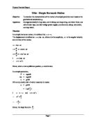
- The acceleration was worked out from the slopes of curve in the velocity-time graph. The corresponding displacement was found. The displacement-acceleration graph and the acceleration-time graph were plotted (on Page 5 and 6 ).
Result:
Data evaluation:
From the displacement-time graph, the curve is a half cycled cosine curve. The curve in the velocity-time graph is a negative, half-cycled sine curve. The curve in the acceleration-time graph is a negative, half-cycled cosine curve. From the acceleration-displacement graph, a straight line was shown, which the acceleration is always in the opposite direction and is directly proportional to the displacement. So we can use the following equation to represent the motion:
a = -w ² x
(where a is the acceleration, w is the angular velocity ( a positive constant ), x is the displacement)
The definition of simple harmonic motion (S.H.M.) is:
- the acceleration of a particle is
- directed towards a fixed point
- directly proportional to its distance from that poing
- the acceleration is always in the opposite direction to the displacement
So, the equation a = -w²x proved that the pendulum performed S.H.M.
Also, for a S.H.M. the angular velocity (w) is kept constant. Period (T) is equal to 2∏/w, so the period is also kept constant and is independent of amplitude and mass of the bob.
From the graphs the value of w is more or less the same within the motion.
As period (T) = 2∏ / w
So the period is also more or less the same within the motion.
Discussion
Background information of simple harmonic motion.
There is a close connection between circular motion and simple harmonic motion. Consider an object experiencing uniform circular motion, such as a mass sitting on the edge of a rotating turntable. This is two-dimensional motion, and the x and y position of the object at any time can be found by applying the equations:
The motion is uniform circular motion, meaning that the angular velocity is constant, and the angular displacement is related to the angular velocity by the equation:
Plugging this in to the x and y positions makes it clear that these are the equations giving the coordinates of the object at any point in time, assuming the object was at the position x = r on the x-axis at time = 0:
How does this relate to simple harmonic motion? An object experiencing simple harmonic motion is traveling in one dimension, and its one-dimensional motion is given by an equation of the form
The amplitude is simply the maximum displacement of the object from the equilibrium position.
So, in other words, the same equation applies to the position of an object experiencing simple harmonic motion and one dimension of the position of an object experiencing uniform circular motion. Note that the In the SHM displacement equation is known as the angular frequency. It is related to the frequency (f) of the motion, and inversely related to the period (T):
The frequency is how many oscillations there are per second, having units of hertz (Hz); the period is how long it takes to make one oscillation.
Velocity in SHM
In simple harmonic motion, the velocity constantly changes, oscillating just as the displacement does. When the displacement is maximum, however, the velocity is zero; when the displacement is zero, the velocity is maximum. It turns out that the velocity is given by:
Acceleration in SHM
The acceleration also oscillates in simple harmonic motion. If you consider a mass on a spring, when the displacement is zero the acceleration is also zero, because the spring applies no force. When the displacement is maximum, the acceleration is maximum, because the spring applies maximum force; the force applied by the spring is in the opposite direction as the displacement. The acceleration is given by:
Note that the equation for acceleration is similar to the equation for displacement. The acceleration can in fact be written as:
All of the equations above, for displacement, velocity, and acceleration as a function of time, apply to any system undergoing simple harmonic motion. What distinguishes one system from another is what determines the frequency of the motion
We choose a 1.5 m long string and the amplitude to be 13 cm because we need to ensure the swing angle is less than 5 º. The restoring force F = ma = - mgsinθ, which always tends to bring the object back to the original (zero) position.
For very small θ,
∴S.H.M.
After studying the x-t, v-t, x-a and a-t graphs , I know more about the phase angle. The following figure shows three instant in the motion of a pendulum.
At H, the acceleration a is maximum and positive. A quarter cycle later, at O, the velocity v is maximum and positive. Another quarter cycle later, the position x is maximum and positive at K. One cycle corresponds to an increase of 2∏ or 360º for Ø. So a quarter cycle corresponds to 1/2 ∏ or 90º. Thus,
-
the acceleration leads the velocity by 1/2 ∏
-
the velocity leads the position by 1/2 ∏
Conversely, the velocity lags the acceleration by 1/2 ∏, and the position lags the velocity by 1/2 ∏. The acceleration and position are out of phase by ∏, i.e. they are in antiphase. These differnences in the value of Ø are called phase difference.
The velocity and acceleration of the bob, just like the displacement, can be described by rotating vectors of magnitude wA and w²A respectively. The relative phase relations, i.e. a leads v by 1/2∏ and v leads x by 1/2∏, are obvious from such a figure.
At H At O At K
The new equations for displacement, velocity and acceleration are as follows:
x = AcosØ
v = -wAsin(Ø + 1/2 ∏ )
a = -w²Acos(Ø + ∏ )
As a = -(g/l)x
w² = g/l
w = (g/l)½
T = 2∏ /w
Period is not only dependent on the swing angle, but also the length of string, while the amplitude and mass do not affect the period. So it is isochronous.
Error Analysis
In this experiment, the errors mainly come from frictions, with air and within the string, as well as the friction between the ticker-tape and the chair. They act as a damping force and slow down the motion. So energy is lost continuously to overcome the fictions. This damping force is directly proportional but in opposite direction to the velocity of the bob. The damping force is equal to –bv where b is a positive constant and v is the velocity of the bob. Now the restoring force is no long equal to mgsinØ. The new equation of restoring is ma = mgsinØ – bv. The expression a = -(g/l)x is no longer be obtained. So the motion is not simple harmonic one anymore.
The swing angle is difficult to keep under 5 º. So if an angle larger then 5 º is used, the equations
cannot be held and so the motion is not a simple harmonic one.
When leave the ringed mass and let it to swing, we may give an external force to it. Also the mass oscillates horizontally during the swinging motion. These may affect the swing angle and the velocity of the bob and this explained why the dots on the v-t graph cannot connect together to form a smooth curve.
Another big problem is to measure the slopes of the curves accurately. This explains why the dots in v-t, x-a and a-t graphs cannot connect together to form smooth curves and straight line.
Improvements
- Hold the mass stationary for a while before leaving it. Try not to exert any force to the mass.
- Twist the clamp as tight as possible so the whole system will not vibrate or oscillate.
- Set the ticker-tape timer at a place which cannot touch the chair, while keeping on the same horizontal plane with the mass.
- use a plane mirror to get the normal of the dots and then calculate the slopes of the dots.
Conclusions
Simple pendulum is a kind of simple harmonic oscillator. The experimental results satisfied the equation for simple harmonic motion ( a = - wx)


