I will plot a graph with axis voltage against current to find the resistance of each wire used, and then use those resistances to plot a graph with axis resistance against
1 / cross-sectional area. I will use this graph to work out the resistivity of the constantan wire.
Preliminary
I used the method and procedure to do the preliminary experiment, to see if I could see some kind of trends in readings, and hence change my prediction, I wanted to use varied variables, so I can get an image of what would happen in each case. The readings I found were as below;
Looking over these results, I think that it is best not to use the 1.25mm diameter wire because the current rose too high and so was potentially dangerous, i.e. it could scold hand at touch.
Thinking about voltages to set the power supply to, I think it would be best to use 13V because if we scale up quantities, in this case, voltage, we, as a result increase the accuracy.
Here we used a wire length of 0.5m, but I feel it would be best to use 1m as it would be easier to work out the resistivity, and it is much more safer because of the increase in temperature as we increase the voltage.
So after this experiment I felt I should use a varied range of diameters of wire, these are listed in the table below:
Fair test
To ensure that I am conducting a fair test, I have decided to take a number of measures to ensure that this occurs.
I am going to use a meter ruler to measure the Constantan wire and ensure that it is the correct length. I am also going to try to ensure that the current is within 0.01Amps of the desired current.
I will also ensure that the thickness of the wire stays constant for each wire by making sure there are no kinks on the wire, which increase the thickness, and I will measure the thickness of the wire at intervals using a micrometer screw gauge.
I will also try to use the same equipment for each current because any change of equipment that might cause a distortion of results.
To make it a fair test, only one factor should be altered at a time. When the constantan wire is being tested, the length and the diameter of the wires should be constant.
Prediction
Taking the content on the previous pages into account, I think that the electrical resistance of a wire would be expected to be greater for a longer wire, less for a larger cross-sectional area and would depend upon the material the wire is made of. So I predict that: -
- If I double the cross sectional area of the wire, then I will cut the resistance by half. This is because a wide wire would allow a high current to pass through it, while it would be more difficult for the current to flow in a narrow wire due to it’s restriction to a high rate of flow.
- The resistance would be higher for a thin wire compared to that of a thick wire because of the increase in collisions of electrons and the metal ions.
Accuracy
I will make my experiment as accurate as I can by using accurate measuring apparatus, such as the micrometer, a digital multi-meter instead of the traditional analogue voltmeter, as the scale divisions are much smaller on the digital meter than on the analogue meters.
I will try to make sure there are no kinks in the wires as this increases the thickness of the wire. I shall measure the diameter from a number of places on the wire so that I can see that the wire is of one diameter on the length.
I will have to take account of possible errors, such as the zero error in equipment, and other random and systematic errors, which can occur.
I will try to avoid making the parallax errors, (the error which occurs when the eye is not placed directly opposite a scale when a reading is being taken). This can be made on reading off a ruler. The reading errors (the error due to the guess work involved in taking a reading from a scale when reading lies between the scale divisions, and the zero error (the error which occurs when a measuring instrument does not indicate zero when it should), which can be possible on the analogue instruments such as the ammeter.
If the zero error happens, then I will adjust the instrument to read zero or the inaccurate zero reading should be taken and should be added or subtracted from any other reading taken. Sometimes the metre rules have worn edges and so I will measure from 10cm instead of 0cm.
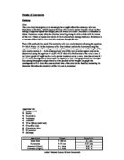
I used a micrometer screw gauge to check that the diameters were correct, because this can affect the results I obtain. I took three readings for each wire, at 0m, 0.50m and 1m.
You can see that the diameters are correct to a certain degree of accuracy, in this case 2.s.f, which makes the experiment a lot more accurate. However, I had found that the wire of 0.90mm in diameter was inaccurate, as it was actually 0.94. There are quite a few reasons to why I had this reading, there could have been an slight zero error, a random error i.e. misreading the scale etc, or the wire may actually be this size due to the manufacturers fault. The manufacturer cannot actually produce a wire which is exactly the size stated.
Reliability
When I am plotting the graph I will make sure that I work with a large scale on the axis, if I plot the graph with resistance against cross-sectional area, I will make sure that I show it to a certain degree of accuracy, maybe 2.d.p. I shall use the most accurate degree of accuracy to work out the resistivity i.e. the cross-sectional area, which has answers which are up to 10 digits long, so I am not going to round the numbers up or down.
Safety considerations
In doing this experiment, I must take many safety considerations into hand. I must make sure that the current flow is not prolonged as the wire will get hot, and thus, increase the resistance in the wire and also to avoid the heating effect, which may burn us or cause damage to surrounding objects. I must also not touch the wire once the power pack is turned on, because I do not know if the wire is hot or not. I must also avoid the wire being exposed to any water on benches, as water is a good conductor, and this could be potentially dangerous.
Prediction Cont
From using my knowledge of errors and the information obtained from sources, I aim to get accurate readings, which will lead me to get an accurate resistivity of the constantan wire. I predict that its graph will show the relationship that resistance is inversely proportional to cross-sectional area, as shown below: -
Obtaining evidence: Results table
Analysis
I used these readings to plot graphs with axis voltage (V) against current (I). These are shown on the following pages.
I then drew a line of best fit for each wire, taking care to even out the number of points on each side of the line and by use of a relatively large scale across the axis.
Having done this, I worked out the gradient of each line, hence the resistance of each wire. This is shown on the graphs.
The graphs drawn are all straight lines, and enter the origin (0,0). These graphs also relate to my prediction, as my predictions states that as the diameter increases, the resistance decreases.
I then placed the calculated resistances (R) in a table with the values of 1/ cross-sectional area (1/A) of each corresponding diameter (D) of wire, as below:
From the table above I can see some trends in my readings, as 1/A increases the resistance increases, this means that as the diameter increases the resistance decreases. This is because with a wire of a small cross-sectional area, it is harder for the free electrons to drift from the negative terminal to the positive terminal. So, there are more collisions between the electrons and the atoms, than in a wire of a larger cross-sectional area.
It is the values highlighted in red in the above table, which I have used to plot the graph, resistance against 1/area, using a relatively large scale across the axis to increase accuracy.
I had used standard form on the x-axis to represent the value of 1/area, because it is easier to plot these values on a graph than using values less than 1.
I also drew a line of best fit in this graph. I used line to find the gradient, which is in fact equal to the resistivity (Ωm) x the length of wire (m). It is to my advantage that the length was 1m because I do not have to divide the gradient by the length. I plotted the graph with x-axis values in standard form to make it easier for me to plot.
*All working of gradients are shown on the graphs.
The graphs fit my prediction, as I predicted that the larger the diameter, the smaller the resistance. My graphs show that a thin wire has more resistance than that of a thick wire. I also see that the resistance of the wires shown in my graph are:
- Inversely proportional to its cross-sectional area.
This can be backed up the resistance equation:
Y = mx + C, where Y is the resistance, m is the gradient of the line, hence, resistivity x length and where C is 1/ cross-sectional area.
After plotting the points on the graph, I worked out the gradient, by using the following formula;
Where, ∆ means Change in…
The value of resistivity of the constantan wire i.e. the gradient of the line was
48.6 x 10⁻⁸Ωm. The calculations of this can be seen on the corresponding graph. This value is close to the accepted value of 49 x 10-8Ωm, as given by “Physics” by Robert Hutchings.
Therefore, the predictions I have made have been substantiated, I have investigated how resistance of a length of wire changes with diameter to determine the resistivity of constantan wire used and I have deduced that resistivity is proportional to 1/A and the resistivity of the wire is 48.6 x 10⁻⁸Ωm.
Evaluation
I feel that I have gained accurate readings, which led me to determine the resistivity of the constantan wire to be 48.60 x 10⁻⁸Ωm. This is accurate to 2.d.p. The resistivity of the constantan wire, as quoted from “Physics” by Robert Hutchings, is 49 x 10-8Ωm at 25ºC, and you can see that I was off by 0.4 x 10⁻⁸Ωm. This difference has occurred because of errors, which could have occurred, by the instruments used and by me, who took the readings.
Having said that, I think that my method in my experiment is accurate to a certain degree, but there were small errors, which led the resistivity to be lower than the actual resistivity. Although there are no major anomalous readings in this experiment, there are certainly a minority of readings, which add to the error. The points on the graphs I drew are close to the lines of best fit.
The points are not exactly in a straight line because the experiment has its limitations and sources of error, some of which are hard to get rid of. For example, the random errors, such as, the misreading of the scale. The systematic error, such as the zero error i.e. an ammeter does not read zero when no current is flowing through it.
However, these errors did not cause major errors in my readings but did account to a small possible change in gradients from graphs.
The percentage errors of the quantities used can be found by using the following formula:
Therefore, I can use this formula to find the percentage error in each quantity I used:
In the table above, I took 1cm to be the absolute error in length because I had to take the fact that the wire was not exactly straight into consideration.
The problems which I experienced with the instruments are, that the multimeter reading would not stay constant, it would move from one voltage to another, i.e. 3.45 – 3.51 – 3.47. As well as this, measuring the length of the wire was quite difficult because to get the measurement closest to 1.00m, you had to make sure the wire was a straight as possible, but if you pull the wire, too much you are as a result, stretching it. This decreases the cross-sectional area, and so the resistance would be higher.
I used seven diameters of wire in total, so that I would have more points to plot on the graph.
As I used an analogue ammeter instead of the digital multimeter, I lost accuracy, and as you can see from the percentage error, of 3.13%, you’ll find that it is much easier of misread the reading than in an digital meter. If I used the digital ammeter instead of the analogue ammeter, I would have decreased the percentage error, hence increase the accuracy of the experiment. I could make this an improvement on my method if I was to do the experiment again. I could use a shorter wire than 1m, to increase the accuracy in the actual measuring of the wire, as it is easier to handle, than a longer wire which is harder to hold down and measure.
Another improvement I could make is to use a stainless steel metre rule. This is because I found that the rulers supplied had worn edges and scale, so an error could be made easily. The steel rule, is much more reliable in measuring the length of wire because it doesn’t ware down easily like wooden metre rules, the divisions are embedded into the steel and so that cannot be worn down as in the wooden rulers.
Taking more readings and repeats increases the accuracy and so I would do this to improve my method, as I had not taken any repeats on this occasion.
The procedure I used to find the resistivity, I felt was reliable, because the points on the graphs were close to the line of best fit, but the thing I done wrong was plot more readings on one graph than on another. This is because I was using random voltages by moving the variable resistor at random intervals, it was hard to get the voltage to remain constant on the digital voltmeter. I had used seven different diameters of wire; hence sustain a range of cross-sectional areas. Though using more wires would have increased accuracy of the final resistivity.
I had calculated the max/min gradients used to find the resistivity; the table below shows my outcomes.
Using the above table, I have to work out the uncertainty in the resistivity.
I found the resistivity of the constantan wire to be 48.60 x 10⁻⁸Ωm.
So if I were to find the uncertainty in the value for the resistivity, I would have to use the following formula: -
However, as the gradient on the graph was equal to the resistivity x length, I have to add the error in length to find the possible error in the overall experiment.
Now, I have to calculate the error from this percentage uncertainty. You do this by calculating 3.29% of the gradient of the line of best fit.
This % Uncertainty of 3.79%, tells me that the procedure or method I used is quite accurate, by looking at the size of the possible error of ± 1.84 x 10⁻⁸Ωm. However, it also tells me that there is some room for improvement, such as repeating readings for accuracy and taking the average. The largest % Uncertainty was in the current, this being because I had used an analogue ammeter, if I had used a digital ammeter, the % Uncertainty would have reduced to 1.56%.
Overall, on looking at the actual resistivity, from “Physics For You”, I believe that my results were accurate, but taking the errors into account there is a possible range in my resistivity being between: 46.76 x 10⁻⁸ Ωm – 50.44 x 10⁻⁸ Ωm. This tells me that the resulting error is a major contribution to the resistivity, as this error can have a huge effect on the resistivity of the constantan wire I used. However, on doing this experiment again, I would know what to look out for, i.e. specific errors, change of equipment, i.e. the steel rule and digital meters.
Bibliography