6. Using the power supply, induce current flow through the circuit.
- Make sure the potential difference across the metal is held constant at 0.30 volts using the power supply settings. Verify voltage constancy with the voltmeter.
- Record the current reading shown on the ammeter, together with the length of metal wire forming part of the circuit.
- Repeat stages 9 – 11 ten times, increasing the distance between the two pairs of alligator clips by 10 cm each time. Doing this increases the metal wire length forming part of the circuit.
- The resistance of the metal wire is obtained by dividing the voltage used in every measurement (0.30 v) by the current measured in every measurement. You should get different resistance values for different lengths of wire used. This calculation assumes the wire to be ohmic.
Results
The method above was conducted. A table comparing the length of the metal wire, its induced current, and its consequent resistance is shown below. Note that the potential difference across the metal wire in all the measurements is 0.30 volts:
*Values for resistance are given to two significant figures - the same as the significant figures for voltage values. Uncertainty in resistance will be calculated later. The resistance was calculated as specified in step 13 in the method.
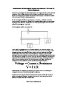
For further investigation, it is necessary to calculate the uncertainty range for the resistance values. As previously mentioned, the resistance of the wire is attainable through the equation R = V/I, if assuming the wire to have ohmic behavior. R is wire resistance, V is potential difference across wire, and I current through wire. The relative uncertainty for resistance is therefore
ΔR/R = ΔV/V + ΔI/I
Hence, the absolute resistance uncertainty is
ΔR = R · (ΔV/V + ΔI/I ).
Since the potential difference, its uncertainty, and the uncertainty in current are constants throughout, then:
ΔR = R · (0.02/0.3 + 0.02/I )
This equation is applicable to the resistance values obtained in the preceding table. Below is a table showing the same resistance values as before, with individual uncertainty for each value. Uncertainties are expressed in two significant figures, just like the actual resistance values. Each value is compared with the respective wire length used:
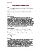
From the data collected, a graph of wire resistance vs. wire length was constructed. It includes error bars for both length and resistance, though the former are too small to be seen. The graph is shown on the next page:
Although one set of data points was plotted, three regression lines were drawn. The one in the middle (Y1) is the regression line for the points plotted. The ones above and below it (Y2 and Y3 respectively) are regression lines that pass through the error bars to give the greatest and smallest possible gradients for the data (i.e. greatest and smallest value of constant k). Note that the three lines of regression do not intersect in their middle as is common. That is because the individual resistance error bars plotted increase with each data point. They don’t stay constant throughout.
The regression line passing through the plotted points has equation y = 0.6358x + 0.0293. The coefficient of correlation of the regression line is approximately 0.999, indicating that the regression line equation is an extremely reliable indicator of the relationship between the resistance and length of the metal wire, based on the experimental results. This relationship seems to be proportional in its nature. However, it is not directly proportional. The regression line does not pass through the origin. It is for this reason that the other possible lines of linear regression come in handy. Through their examination, alternative y- intercepts could be searched for in hope of substantiating the direct proportionality relationship sought after. The equation dominating Y2 is y = 0.7x + 0.02. Concurrently, Y3 is dominated by equation y = 0.5222x + 0.0578. Both equations represent linear regression lines that do not pass through the origin, but above it. They intersect the Y – axis at positive values. No matter how one examines this data, the metal wire seems to contain electric resistance when it has no length, which is a debatable result. The existence of a systematic error in the experiment is a more sensible conclusion.
Conclusion
The experiment yielded results that point at a proportional relationship between the length of the metal wire, and its electric resistance. As hypothesized, increasing wire length means increasing its electrical resistance. The linear line of regression passing through the plotted data points substantiated this. The two extreme linear lines of regression fitted to the error bars also reinforced the linearity. In all cases, a linear, or proportional, relationship appears to exist between the variables examined. The constant of linear proportionality, k, fluctuates from 0.52 Ωm-1 to 0.7 Ωm-1, depending on the error bars used.
The results of the experiment, however, do not adhere to the direct proportionality relationship predicted in the hypothesis. In the hypothesis a zero value for wire length is predicted to induce a zero value for wire resistance. Intuitively, this should be the case. However, regardless of what linear line of regression one examines from the ones plotted, it is obvious that the experiment indicates the existence of electric resistance even when the wire has no length. This result is indicated through the intersection of the regression curves with positive Y – values. The ‘zero – length’ resistance varies from 0.02 to 0.0578 ohms. The existence of errors in the experiment, namely systematic ones, may help explain the result.
Errors
The method for the experiment contained some errors. Some of those are evident when examining the results of the experiment. Others are very small, and did not have a great effect on the final outcomes.
The most prominent source of error had to do with the existence of additional resistance in the circuit used. The metal wire used, since it wasn’t a wire meant for electrical circuits, naturally offered the greatest resistance to current flow. Nevertheless, the connecting wires also contained some inevitable resistance. Additionally, the ammeter, and power supply also had some internal resistance (the voltmeter did as well, but this is necessary for the procurement of accurate voltage values). Since current flowed through all those, the resistance values obtained did not represent solely the resistance of the metal wire. This probably explains the systematic error foreboded in the conclusion. The existence of resistance in other pieces of apparatus except the metal wire allowed for the possibility of resistance even when the metal wire would have no length.
Another source of error existed in the measurement of the wire length used in the circuit. The metal wire used was manipulated to assume a straight form. However, even after it was firmly attached to a table, it was not fully stretched. In some of the cases, it may have bent slightly, making the total wire length greater than what was measured. This could have contributed some additional, and unwanted, resistance to the wire. After all, a longer wire offers more resistance to current flow. Altogether, an addition to the systematic overestimation of the resistance of the metal wire also came from this error source.
Though negligible, some error could have sprung from the heating of the wire used. As current was allowed to flow through the metal wire, atoms of the wire collided with the electrons flowing, causing the wire to heat up. If the wire weren’t allowed to cool down before another measurement was taken, then it would have posed additional resistance to the subsequent current flows, since resistance rises with temperature. Again, the method used in this experiment allowed for the existence of additional resistance in the wire that was not taken into account.
Improvements
In light of the errors noted, or for the need to perfect other experiments of the same type, improvements to the method can be offered.
Firstly, the error involving the length of the metal wire could be minimized in two ways. Either a much more flexible wire could be used for the allowance of a straighter metal wire, or a greater effort could be made to stretch the existent wire so that it is much more straight. In both ways, the length measured for the metal wire would be more representative of the actual length being used.
Another improvement could deal with minimizing the existence of additional resistance in the circuit besides that of the metal wire examined. This could be done in several ways. The connecting wires used could be shorter, meaning their resistance would be smaller. A power supply and ammeter with smaller internal resistances could also be used. In either of the cases, additional resistance in the circuit would decrease, and the systematic error in resistance minimized.
Finally, though not too necessary, it is possible to improve the experiment by minimizing resistance distortions due to temperature increases. A simple way would be to wait at least 3 minutes between each current flow induced through the wire. This way, the whole circuit together with the wire itself would have time to cool down. Wire temperature would hence not be a factor distorting the resistance values being measured, as it would be more or less the same in all measurements. Nevertheless, it may be that the distortions to resistance values caused by temperature increase are so small that this improvement on the whole is futile.
Another minor improvement to the method would be the use of a switch. This way, current flow could be initiated and stopped on demand (i.e. immediately). It would be of course necessary to use a switch that offers little resistance. Otherwise, the current construction of the circuit is preferable.