When looking at all three functions on one graph, we see the following:
In order to find the equation of the inverse exponential graph 𝒚=,𝒆-−𝒙., we will use simultaneous equations. And for 𝒚=,𝒙-−𝟏., we will use the autograph system via trial and error.
𝒚=,𝒆-−𝒙.
To create a model for the inverse exponential graph, we can use simultaneous equations. We need to create two different constants, and use information from the table to ascertain the equation. So, by using 𝒚=𝒂,𝒆-−𝒙.+𝒃 and finding 𝒂 and 𝒃 (the two constants), we should be able to form a fairly accurate equation. (We should note that all values will be rounded up to 3 decimal places depending on the value).
We should take the first and last sets of data from the table, and substitute them as ,𝒙,𝒚.. Then substitute those values into 𝒚=𝒂,𝒆-−𝒙.+𝒃.
So ,𝟏.𝟕,𝟒𝟐. is plugged into 𝒚=𝒂,𝒆-−𝒙.+𝒃 to form the first equation, 𝟒𝟐=𝒂,𝒆-−𝟏.𝟕.+𝒃
We should do the same with the last set of data, ,𝟏𝟑.𝟗,𝟑.𝟐.. So after plugging that into 𝒚=𝒂,𝒆-−𝒙.+𝒃, we get the second equation, 𝟑.𝟐=𝒂,𝒆-−𝟏𝟑.𝟗.+𝒃.
We should subtract the first equation from the second equation in order to find 𝒂 and 𝒃. So, ,𝟒𝟐=𝒂,𝒆-−𝟏.𝟕.+𝒃.−,𝟑.𝟐=𝒂,𝒆-−𝟏𝟑.𝟗.+𝒃..
,𝟒𝟐−𝟑.𝟐=𝒂,𝒆-−𝟏.𝟕.−𝒂,𝒆-−𝟏𝟑.𝟗.+𝒃−𝒃.
𝟑𝟖.𝟖=𝒂𝟎.𝟏𝟖𝟑
𝒂=𝟐𝟏𝟐.𝟎𝟐𝟐
Now we should substitute the new value of 𝒂 into either the first or second equation.
𝟑.𝟐=,𝟐𝟏𝟐.𝟎𝟐𝟐𝒆-−𝟏𝟑.𝟗.+𝒃
𝒃=𝟑.𝟐
Therefore, 𝒚=𝟐𝟏𝟐.𝟎𝟐𝟐,𝒆-−𝒙.+𝟑.𝟐
The below graph consists of my model 𝒚=𝟐𝟏𝟐.𝟎𝟐𝟐,𝒆-−𝒙.+𝟑.𝟐 versus the original ‘large nut’ graph
My model does not have as steep a descent of that of the original ‘large nut’ graph and the curve of my graph drops to just below that of the original’s, but then equalizes with the original at the point ,𝟏𝟑.𝟗,𝟑.𝟐.. In my model, the asymptote matches that of the original’s exactly on the 𝒙−𝒂𝒙𝒊𝒔, but not on the 𝒚−𝒂𝒙𝒊𝒔. My model crosses on 3 points of that on the original; ,𝟏.𝟕,𝟒𝟐., ,𝟒.𝟏,𝟔.𝟖., and ,𝟏𝟑.𝟗,𝟑.𝟐.. Though there are some similarities, the results are not particularly satisfying. So, we will use the trial and error method with 𝒚=,𝒙-−𝟏. which will result in a more accurate answer, because since we will be using more parameters, we will be able to shape the equation more closely to the original ‘large nut’ graph.
𝒚=,𝒙-−𝟏.
By using the method of trial and error, we will estimate an approximately accurate model to the original ‘large nut’ graph. We will manipulate the function by using the following format:
𝒚=,𝒄(𝒙+𝒅)-−𝟏.+𝒆
𝒚=,𝒙-−𝟏.
We will increase the value of 𝒄 in 𝒚=,𝒄(𝒙+𝒅)-−𝟏.+𝒆
𝒚=𝟐𝟎(,𝒙-−𝟏.)
We will increase the value of 𝒄 in 𝒚=,𝒄(𝒙+𝒅)-−𝟏.+𝒆
𝒚=𝟐𝟖(,𝒙-−𝟏.)
We will increase the value of 𝒄, and decrease the value of 𝒅 in 𝒚=,𝒄(𝒙+𝒅)-−𝟏.+𝒆
𝒚=𝟐𝟖(,𝒙−𝟏.𝟎𝟒)-−𝟏.
We will decrease the values of 𝒄 and 𝒅 and increase the value of 𝒆 in 𝒚=,𝒄(𝒙+𝒅)-−𝟏.+𝒆
𝒚=𝟐𝟏.𝟕(,𝒙−𝟏.𝟏𝟑)-−𝟏.+𝟏.𝟒𝟓
We will decrease the value of 𝒄 and increase the values of 𝒅 and 𝒆 in 𝒚=,𝒄(𝒙+𝒅)-−𝟏.+𝒆
𝒚=𝟏𝟖.𝟕(,𝒙−.𝟑𝟕)-−𝟏.+𝟏.𝟕𝟖
We will decrease the values of 𝒄 and 𝒆 increase the value of 𝒅 in 𝒚=,𝒄(𝒙+𝒅)-−𝟏.+𝒆
𝒚=𝟏𝟐.𝟕(,𝒙−𝟏.𝟑𝟖𝟒)-−𝟏.+𝟏.𝟕𝟔
We will increase the values of 𝒄 and 𝒆 decrease the value of 𝒅 in 𝒚=,𝒄(𝒙+𝒅)-−𝟏.+𝒆
The Final Result: 𝒚=𝟏𝟐.𝟗𝟏(,𝒙−𝟏.𝟑𝟕)-−𝟏.+𝟐.𝟐𝟏
In the function, we can see that the shape is very similar to that of the original. Though, the function 𝒚=𝟏𝟐.𝟗𝟏(,𝒙−𝟏.𝟑𝟕)-−𝟏.+𝟐.𝟐𝟏 doesn’t run through any point as accurately as 𝒚=𝟐𝟏𝟐.𝟎𝟐𝟐,𝒆-−𝒙.+𝟑.𝟐, the properties of the graph (area under the curve) will be more similar.
In order to get truly determine the more accurate function, we need to compare the graphs to each other. The following graph displays 𝒚=𝟐𝟏𝟐.𝟎𝟐𝟐,𝒆-−𝒙.+𝟑.𝟐 as the purple line and 𝒚=𝟏𝟐.𝟗𝟏(,𝒙−𝟏.𝟑𝟕)-−𝟏.+𝟐.𝟐𝟏 as the blue line.
The biggest difference between the graphs is that 𝒚=𝟏𝟐.𝟗𝟏(,𝒙−𝟏.𝟑𝟕)-−𝟏.+𝟐.𝟐𝟏 has a reflected graph across, onto the negative axis. And as we can see on the above graph, the original ‘large nut’ graph function isn’t reflected. This is because there cannot be a negative height or a negative number of drops.
If we take a close up for the graph (only the positive axis), we will see the following:
One difference is that the inverse exponential 𝒚=𝟐𝟏𝟐.𝟎𝟐𝟐,𝒆-−𝒙.+𝟑.𝟐 is not quite as steep as the original ‘large nut’ graph, however 𝒚=𝟏𝟐.𝟗𝟏(,𝒙−𝟏.𝟑𝟕)-−𝟏.+𝟐.𝟐𝟏 is as steep.
We can also see here that 𝒚=𝟐𝟏𝟐.𝟎𝟐𝟐,𝒆-−𝒙.+𝟑.𝟐 crosses the 𝒚=𝒂𝒙𝒊𝒔 at approximately (𝟎,𝟐𝟏𝟓), which shows a clear limitation to the graph. On the other hand,
𝒚=𝟏𝟐.𝟗𝟏(,𝒙−𝟏.𝟑𝟕)-−𝟏.+𝟐.𝟐𝟏 shows that it has 2 asymptotes – 1 on each axis. This thereby, portrays the original 'large nut' graph with more accuracy.
And, 𝒚=,𝒙-−𝟏. has a more similar area under the curve than 𝒚=,𝒆-−𝒙..
Area under the curve of the original ‘large nut’ graph:
74.91
Area under the curve of 𝒚=𝟏𝟐.𝟗𝟏(,𝒙−𝟏.𝟑𝟕)-−𝟏.+𝟐.𝟐𝟏
73.913
Area under the curve of 𝒚=𝟐𝟏𝟐.𝟎𝟐𝟐,𝒆-−𝒙.+𝟑.𝟐
77.773
And because 𝒚=,𝒙-−𝟏.’s area under the curve is closer to the original’s, it is more similar.
Now, let us apply the function that is most similar to our original graph 𝒚=𝟏𝟐.𝟗𝟏(,𝒙−𝟏.𝟑𝟕)-−𝟏.+𝟐.𝟐𝟏 to other models of different sized nuts.
Medium Nuts
Graph showing the medium nuts (red line) versus 𝒚=𝟏𝟐.𝟗𝟏(,𝒙−𝟏.𝟑𝟕)-−𝟏.+𝟐.𝟐𝟏
(blue line)
We will manipulate the graph (via the trial and error method) by manipulating the function in the 𝒚=,𝒄(𝒙+𝒅)-−𝟏.+𝒆 format.
We need to increase the value of 𝒄 and decrease the values of 𝒅 and 𝒆 in 𝒚=,𝒄(𝒙+𝒅)-−𝟏.+𝒆
𝒚=𝟑𝟎(,𝒙−𝟏.𝟖𝟑)-−𝟏.+𝟏.𝟓
Small Nuts
Graph showing the medium nuts (red line) versus 𝒚=𝟏𝟐.𝟗𝟏(,𝒙−𝟏.𝟑𝟕)-−𝟏.+𝟐.𝟐𝟏
(blue line)
We will manipulate the graph (via the trial and error method) by manipulating the function in the 𝒚=,𝒄(𝒙+𝒅)-−𝟏.+𝒆 format.
We need to increase the values of 𝒄 and 𝒆 and decrease the value of 𝒅 in 𝒚=,𝒄(𝒙+𝒅)-−𝟏.+𝒆
𝒚=𝟐𝟏.𝟔𝟓(,𝒙−𝟑.𝟓𝟕)-−𝟏.+𝟔.𝟗
We are only able to get the general shape because of the structure of the original data points, which does not make very accurate. The limitations of the model is that it is done by trial and error. So it will never be exact no matter what we do to improve it. Also, because of the irregularity of the line graphs of the small and medium nut graphs, the models will never be able to fully replicate them. The medium and small nut graphs are not real curves, and because the models that have been created will always be curves, it will be impossible to create an ideal graph.
The function 𝒚=𝟏𝟐.𝟗𝟏(,𝒙−𝟏.𝟑𝟕)-−𝟏.+𝟐.𝟐𝟏 does not particularily depict the medium and small nut graphs very well. However, by using the method of trial and error, we have been able to manipulate the graphs into the general shape of the original graphs. As said earlier, an ideal graph will never be created, but by this method the slope, area under the curve, and other properties will be similar to that of the originals’. A limitation is that the graph will continue almost straight up. In reality and in the medium and small nut graphs, as the height of the drop (𝒚−𝒂𝒙𝒊𝒔) decreases so will the number of drops (𝒙−𝒂𝒙𝒊𝒔). In this case, the models will never work.