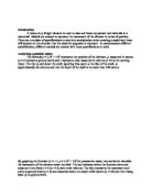
The chart below shows the position of the elevator at different times:
By changing to function mode, we can take a better look at the position, velocity, and acceleration of the elevator.
Position Function:
In the position graph above, we see that the elevator starts at ground level, reaches a height of 80 meters below, and goes back up to up to ground level, all in the course of 6 minutes.
Velocity Function:
By taking the derivative of the position function (y = 2.5t3 − 15t2), we get the velocity function of y = 7.5x2 – 30x. Velocity is the rate of change in position of the elevator. In the velocity graph, we see that the negative velocity means that the elevator is below ground level, which is arbitrarily labeled as y = 0. The velocity function matches the position function in indicating that the elevator goes down and then goes back up. The zero value of the velocity graph means that the elevator is stopped. The negative value means it is moving down away from ground level and the positive value means that it is going up moving towards ground level.
Acceleration Function:
The above graph indicates that the acceleration is increasing constantly. Acceleration is the rate of change in velocity. As the elevators goes down and up, acceleration goes from negative to positive since the velocity is constantly changing. Acceleration is negative while the velocity is decreasing and the elevator moves down. Acceleration is positive when the velocity increases and the elevator changes direction. When the elevator is at rest, the velocity is zero but the acceleration is still increasing since that just means it had increased to zero from negative velocity. When the elevator speeds up, velocity is increasing as acceleration is increasing. When the elevator slows down, velocity decrease as acceleration decreases.
The above model is a fairly good model of the movement of the elevator. However, a couple of issues arise. The model never descends all the way to 100 meters below the ground and only reaches 80 meters, which is not accurate since it makes no sense that the elevator does not go to all the heights it should reach. Also, the model does not allow for stops which the elevator is bound to make.
Creating a new model
When creating a new model for the freight elevator, one must take in consideration several different specifications such as at what height the elevator starts. Also, the speed of the elevator and ways to account for the stops of the elevator must be included for the specifications of the new model.
The new model is the piecewise function below:
y = { 50sin(π/2 x + π/2) – 50, when 0 ≤ x < 2
−100, when 2 ≤ x ≤ 3
50sin(π/2) – 50, when 3 < x ≤ 5
The first function shows the descent of the elevator. The second part of the piecewise function indicates that the elevator has stopped for a minute, for something such as loading or unloading. Finally, the last part shows the elevator going back up to ground level.
y = { 25πcos(π/2 x + π/2) , when 0 ≤ x < 2
0, when 2 ≤ x ≤ 3
25πcos(π/2 x) , when 3 < x ≤ 5
The above graph shows the velocity of the elevator. It decreases and increases as the elevator goes down. The flat section shows the time when the elevator is stopped. Then the velocity increases and decreases as it goes up.
y= { -25π2/2 sin(π/2 x + π/2) , when 0 ≤ x < 2
0, when 2 ≤ x ≤ 3
-25π2/2 sin(π/2 x) , when 3 < x ≤ 5
The above graph shows the acceleration of the elevator. It increases as the elevator goes down, halts when the elevator is stopped, and then decreases as the elevator goes back up.
This is just one model of the movement of the elevator as in moves up and down. The features of this model can be easily modified to fit other situations as well. By adding or subtracting a value to the term inside sin, one can move the curve left or right. This way, one can determine at what level the elevator starts at. In the model, it starts at ground floor. However, this can be adjusted to start anywhere between y = 0 and y = 100. The number in front of the sin term determines the altitude and in turn how far down the elevator goes. For a different freight elevator, this number could to adjusted to fit how far that elevator will travel. The term in sin also determines the period, which would be how long a trip up and down would take. In the case of my model, the trip would take 4 minutes without any stops. This value multiplied by the variable determines this and can be changed to make the elevator go faster or slower. Making the model a piecewise function allows for sudden stops, which is hard to model in a single continuous function.
Applying the model
This model may be further modified to fit a number of other situations. It can represent the up and down movement of other objects in life such as an airplane or rocket. One can use the strategies mentioned above to modify the period, altitude, and maximum and minimum to fit the situation that it calls for.