Now we need to use the matrix method again to find a cubic equation that will model the specified data. A cubic equation is: ax3+bx2+cx+d, and to solve for it, the matrices will have to be in the dimensions 4 by 4 and a 4 by 1. So the first thing I had to do was to split the data into two different matrices, so I did one group of data the odd x’s and one group the even x’s.
Odd Even
Now plug each of the x’s into the cubic function (ax3+bx2+cx+d). Then put each group of data into a 4 by 4 matrix and set the y values into a 4 by 1 matrix.
For Odds:
x =
[A] [x] [B]
For evens:
x =
[A] [X] [B]
At this time, use the process x to solve for [X]. After doing so:
Odd: [X]= Even: [X]=
Then put each of the variables into a cubic function format and generate a graph for each equation.
The odd: f(x)=.0416666667x3 +.625x2 +10.9583333x-1.625
This graph shows that it touches all the data points, except when x=6. This equation models the given data by almost passing every point.
The even: f(x)= .0625x3 +.375x2 +12x -3
This graph illustrates that all, but the sixth point is touched by this function. Although this function is different from the odd cubic function, they both go through the same points and not the sixth. The differences of these two graphs are only the different numbers written for the cubic function.
Next, we need to create a polynomial function that passes through all of the particular data. To do this, I decided to create a polynomial function by using matrices. In order to use matrices, we need to make the dimensions the same. Hence, we are given eight precise data points and to solve for a function, we need to make an 8 by 8 matrix and an 8 by 1 matrix. In order to create these dimensions, we need to set up a format for the polynomial function. As a result I set up the first term/part to be ax7, the second bx6, and so on so forth. To construct the 8 by 1 matrix, I used the letters of the alphabet a through h. Then, by using the format ax7+ bx6 +cx5 +dx4 +ex3 +fx2 +gx +h, I created my 8 by 8 matrix.
x
[A] [X] [B]
Now take the x to solve for [X]. Using a graphing calculator, enter what each of the variables are into a equation and press “GRAPH.” The equation is supposed to be:
f(x)=.0025793651x7 - .0777777777x6 +.95555552x5 – 6.152777775x4 +22.25138888x3 -43.76944443x2 +55.79047617x – 18.999999999
Looking at this graph it shows that this function fits all the points except the sixth. There seems to be a hitch on getting a function that would go through the sixth point throughout this investigation so far. There seems to be no difference between the cubic functions created by matrices and this polynomial function.
Our last method is using technology to help find another function that fits this data. By using a graphing calculator, enter the data into the calculator’s lists. Press the STAT key and choose option 1: Edit from the Edit screen. This will bring up the List screen, and input all the data put the x-values data in list L1 and put your y-values data in list L2. Then, turn on plot 1 from STATPLOTS. Next, I set my windows to fit my data. Now that we have our scatter plot, we need to figure out a equation or two that will model all of the given data points.
To find a quadratic equation, press STAT and go to CALC and go down until QuadReg is seen, then press enter. After doing so, the calculator will give you what a, b, and c is equal too. So the equation is: 1.244047619x2 + 8.458333333x + .8392857143. The graph is:
Also by finding the QuadReg, it gives you what r2 is. And for this equation, the regression is .99982635. This function models the data very well beside the third point.
To find a cubic equation, all I did was press CubicReg instead of the QuadReg, and I got the function to be: .0631313131x3+.3917748x2+11.70959596x -2.285714286. The graph looks like this:
The regression for this function is .99996999372. This regression is greater than the regression from the QuadReg, which indicates the cubic function is stronger and fits the data more closely. This function models the data like the functions created by using matrices because it doesn’t go through the sixth point.
Now using LinReg(ax+b) in the calculator, will allow us see the regression and equation of the line. The equation is y=(19.65)x+(-17.81) with the regression .98
And the graph is:
I think the function from the CubicReg best models the given data because the regression is very closer to 1 than the QuadReg. The quadratic equation from the matrix method fails to connect to more than one point. The cubic functions from created by the matrix method models the data just like the CubicReg, but there are so many different ways to split the data into two sets of fours, and my method was just one way. The polynomial function modeled the data quite well, but since the CubicReg and polynomial function both missed one point, the function with the larger regression got to be the better function. So the function, 0631313131x3+.3917748x2+11.70959596x -2.285714286 models the data the most precise.
After creating functions, we need to choose a quadratic model to decide where to set a ninth guide. Using the quadratic function made from the use of technology, I set x=9.
1.244047619x2 + 8.458333333x + .8392857143 (x=9)
=100.7678571 + 76.07999997 + .8392857143
=177.7321429
The ninth guide could be placed 170cm from the tip of the fishing rod. By adding this ninth guide, it permits another possible quadratic function by using the last set of 3 data points, since we have already used the first and second set of 3 data points. See below:
By adding a ninth guide, it will affect the all the functions created. The cubic equations would not be as precise since there are an odd number of points. The polynomial equation must begin with ax8 instead of ax7.
Then the assignment gave us a new set of data to compare with the quadratic model from the first part of this investigation. This time Mark has a fishing rod that is 300cm.
The quadratic model fits this data by only going through the first two points, and misses the rest. The quadratic model from the first part of the investigation doesn’t really model this new set of data. To find how to modify the quadratic equation, I used technology to figure out what the QuadReg was and subtracted the first quadratic model by this QuadReg:
1.244047619x2 + 8.458333333x + .8392857143 Original function
- .9345238095x2 + 7.720238095x + 2.05351429 New function
.3095238095x2 + .738095243x -1.214228547
So, the quadratic has to modify by .3095238095x2 + .738095243x -1.214228547 to fit the data created by the 300cm rod. The regression of the function 9345238095x2 + 7.720238095x + 2.05351429, is .9997802355. The LinReg of this data is written y=(16.13)*x+(-11.95 ) with the regression (.99).
The limitations to this model is that there is can’t be an infinite number of guides and rod have only have certain lengths.