-
P= -0.75Q + c
-
3 = -0.75(4) + c
-
3 = -3 + c
- C = 6
So now, we are completely sure that the linear demand equation (P = -0.75Q + 6) for quarter 1 is correct.
Moving onto the 2nd, 3rd and 4th quarters, we can apply the same method of finding the gradient, then substituting the values with P and Q in order to get the linear demand equation.
Calculations to get Linear Demand Equations for 2nd, 3rd and 4th quarters:
We can test its validity by inserting other points to ensure that these linear demand equations are correct,
If we get the same equation we then know that our equations are accurate.
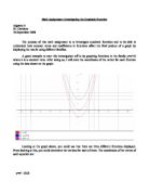
From these justifications, it is clear that our final linear demand equations for all quarters are accurate. The graph below shows all of the final linear demand equations for all four quarters.
Figure 1: Graph showing Linear Demand Equations for all four quarters.
Part 2:
In this section, we will be using the demand equations found in part 1 in order to show the revenue for each of the four quarters. Revenue is the income the company gets, therefore the general equation for revenue is: R= PQ (Revenue= price x quantity). As we know the price (P) already from the linear demand equations, we simply need to multiply everything by Q to get the functions for the revenue.
Calculations:
Quarter One:
- Revenue Equation: R=PQ
- P=-0.75Q+6
- R=(-0.75Q+6)(Q)
Quarter Two:
- Revenue Equation: R=PQ=
- P=-1.25Q+4.5
- R=(-1.25Q+4.5)(Q)
Quarter Three:
- Revenue Equation: R=PQ
- P=-2Q+4
- R=(-2Q+4)(Q)
Quarter Four: P=-Q+6
- Revenue Equation: R=PQ
- P=-Q+6
- R=(-Q+6)(Q)
Now since we have our revenue functions (seen as quadratic functions) we can graph the functions to investigate whether the results make sense and seeing the benefits and limitations to the VBGC.
Figure 2: Graph showing the revenue functions for all four quarters.
From looking at the graph, it can be seen that these parabolas are very different implying that the revenue for each quarter is different, fluctuating throughout the year. Based on the information provided, the VBGC stated that the vast majority of its sales involve selling natural gas to consumers who use it for heating of homes and businesses. In relation to the graph this makes sense as quarters 1 and 4 have the highest revenue since they are the winter months where it is naturally colder. For quarters 2 and 3, as these are the Spring and Summer seasons, this is also logical that the revenue decreased significantly as these are warmer months and gas for heating simply not needed. Also this graph makes sense in relation to economics as the quantities of the gas provided differ for each quarter. Since the winter months are usually colder, the quantity demanded for each will be much higher and even if the company increases its prices people will still pay for gas resulting in higher revenue. In the warmer months, it can be seen that the company significantly reduces the prices and the quantity demanded is much less, which also makes sense otherwise the company would be left with a surplus of gas resulting in a loss of profit.
This graph also does not make sense since all of the parabolas continue into the negatives of price and quantity implying that there would be negative price and negative quantity, which just does not make sense in relation to real-life context. When looking at the concept of supply and demand, it is known that supply can never be negative otherwise the theory would not work, as companies do not sell products if they don’t gain a profit. Also the lowest digit for quantity demanded could reach would be 0 indicating no demand for the good.
In summation, this graph does make sense to an extent if we manipulate it and refine the lines. As proven, the lines of the parabolic graphs cannot go into the negatives however if we restrict and end the lines at the x-axis then this can be a suitable model for real-life situations.
Part 3:
In this next part of the investigation, using our revenue functions from part 2, we will determine the price that the VBGC will need to charge each quarter in order to maximize their revenue. In order to do so, we need to locate the price and quantity, which maximized revenue on the demand curve. In relation to quadratic functions (y= ax2 + bx + c) the easiest way to locate the highest or lowest points of a parabolic graph is to locate the vertex. In this case, we can locate the x-value of the demand curve by using the general equation , which will give us the x-coordinate, then simply substitute the x-value into the linear demand equation to get the value of y. Below is my working out to get the vertex (maximum revenue) and to ensure validity and accuracy, I also inserted my equations into my GDC to ensure my results are correct.
Finding the vertex:
Using quarter 1 as my example, I need to make the function into a quadratic function by getting rid of all the parentheses by utilizing the FOIL method.
- R=(-0.75Q+6)(Q)
-
R=-0.75Q2 + 6Q
Now as we have a quadratic function, we need to convert the equation into terms of a and b in order to utilize the general equation of locating the x-value.
↓ ↓
Now since we know that -0.75 is our a-value and 6 is our b-value, we can simply insert both values into the equation to get our x-value.
We have the x-coordinate of the vertex; we simply need to insert this value into the linear demand equation to find the y-value then we will have the location of the price and quantity, which maximized revenue for the 1st quarter.
- P = -0.75Q + 6
- P = -0.75(4) + 6
- P = -3 + 6
- P= 3
- Vertex: (4, 3)
As a result, we are left with the vertex (4, 3), which is the location of the price and quantity, which maximized the revenue for the 1st quarter. We can determine the price from this since we have the y-value, which is in this case 3 therefore the price that the VBGC will need to charge is 3 Euros per cubic meter in order to maximize their revenue. This can also be shown graphically on figure 3.
Figure 3: Graph showing the maximum revenue for Quarter 1.
We have figured out the maximum revenue for the 1st quarter but we can also apply the same methods to all the other quarters and test them graphically to ensure that the maximum revenues meet and make sense.
Calculations for the Maximum Revenue:
Now we have all of the vertexes for each of the four quarters as well as the price that the VGBC will need to charge in order to maximize their revenue. We can lay this out graphically to ensure our calculations are correct and accurate.
Figure 4: Graph showing the maximum revenue for Quarter 2.
Figure 5: Graph showing the maximum revenue for Quarter 3.
Figure 6: Graph showing the maximum revenue for Quarter 4.
Part 4:
In economics, all firms face another factor called elasticity when dealing with revenue. Elasticity (η) is defined as the responsiveness of demand to changes in quantity demanded as price changes. It can be written in an equation like this:
η = = = = =
Now since we have our elasticity equation, we can simply just focus on the part of the equation and enter the slope, price and quantity of the various demand curves and the maximum revenue in order to get the elasticity.
Calculating Elasticity for Quarter 1.
Using the data points given in the market data table, we can figure out the elasticity by inserting the different prices and quantity demanded from the 1st quarter into the elasticity equation.
- == -3
In this case for every 1% increase in price, the quantity demanded will fall by 3% and the quantity demanded will be seen as highly responsive to price changes or also known as elastic.
- = = -1
In this case, this indicates that for every 1% increase in price, the quantity demanded will fall by 1% and the quantity demanded will have no sensitivity to price changes indicating that it is unit elastic.
- = = -0.33
In this case, for every 1% increase in price the quantity demanded will fall by only -0.33% meaning that the quantity demanded is not very sensitive to price changes therefore it is inelastic.
Calculating Elasticity for Quarter 2.
Using the data points given in the market data table, we can figure out the elasticity for the 2nd quarter by inserting the different prices and quantity demanded into the elasticity equation.
- = = -2.6
In this case for every 1% increase in price, the quantity demanded will fall by 2.6% and the quantity demanded will be seen as quite responsive to price changes or also known as elastic.
- = = -0.8
In this instance for every increase by 1% in price, the quantity demanded will drop by 0.8% and the quantity demanded will be seen as not very responsive to price changes or inelastic.
- = = -0.2
In this instance for every increase by 1% in price, the quantity demanded will drop by 0.2% and the quantity demanded will be seen as not very responsive to price changes or inelastic.
Calculating Elasticity for Quarter 3.
Using the data points given in the market data table, we can figure out the elasticity for the 3rd quarter by inserting the different prices and quantity demanded into the elasticity equation.
- = = -3
In this case for every 1% increase in price, the quantity demanded will fall by 3% and the quantity demanded will be seen as highly responsive to price changes or also known as elastic.
- = = -1
In this case, this indicates that for every 1% increase in price, the quantity demanded will fall by 1% and the quantity demanded will have no sensitivity to price changes indicating that it is unit elastic.
- = = -0.33
In this instance for every increase by 1% in price, the quantity demanded will drop by 0.33% and the quantity demanded will be seen as not very responsive to price changes or inelastic.
Calculating Elasticity for Quarter 4.
Using the data points given in the market data table, we can figure out the elasticity for the 4th quarter by inserting the different prices and quantity demanded into the elasticity equation.
- = = -3
In this case for every 1% increase in price, the quantity demanded will fall by 3% and the quantity demanded will be seen as highly responsive to price changes or also known as elastic.
- = = -1
In this case, this indicates that for every 1% increase in price, the quantity demanded will fall by 1% and the quantity demanded will have no sensitivity to price changes indicating that it is unit elastic.
- = = -0.9
In this instance for every increase by 1% in price, the quantity demanded will drop by 0.8% and the quantity demanded will be seen as not very responsive to price changes or inelastic.
Now we have all of the elasticity’s for the various demand curves from the market table. To find the elasticity of the maximum revenue we simply have to substitute the price and quantity values with the vertexes we found in part 3 in order to get the elasticity.
Calculating Elasticity at the four price and quantity combinations that maximized revenue.
Part 5:
For this last section of the investigation, referring back to my results in parts 3 and 4 I will state the general result about the location on the demand curve for the price and quantity combination in order to find the maximum revenue and the location of this point on the demand curve. I will also state a general result of the elasticity of demand at the point on the demand curve when the revenue of the firm is maximized.
Location on the demand curve for price and quantity combination that will maximize revenue.
Referring back to part 3, in order to find the maximum revenue we had to use the revenue functions and expand out the brackets in order to get the quadratic functions. It can be explained in algebra like below:
- R = PQ
- R = (mQ+c)(Q)
-
R = mQ2+cQ
Now as we have the quadratic function by substituting the value of P with the linear demand equation and expanding out the brackets, we can utilize the general equation of that will locate our x-value, the first part of locating the maximum revenue on the demand curve. Since we are using variables related to the quadratic equation, in order to make things simpler we can substitute b with c from the straight-line equation as they are y-intercepts and a is equivalent to the slope. This can be shown through algebra.
From this equation we can always derive our x-value. It simply has to be substituted into the straight-line equation, resulting with the y-value and our final vertex for the location of the maximum revenue.
- P=m()+c
- P=-+ c
- P=
- (Quantity, Price)= (, )
When we substitute the x-value back into the straight-line equation, and we eliminate the terms we are left with as our y value. We can also prove that these work by taking two points from the market table and seeing if the results match the vertex. For example:
- (Quantity, Price)= (, )
-
= = 4
- = = 3
(Quantity, Price) (4, 3) This clearly proves the general rule as we derive back to the maximum vertex to find the location on the graph of the maximum revenue.
Result of the elasticity of demand when revenue is maximized.
Referring back to part 4, the elasticity’s for the various demand curves will fluctuate as they depend on seasonal changes and the demand at the time of year. For the maximum revenue, we can derive a general rule that will always prove that the elasticity is always unit elastic. This can be presented in algebra if we substitute the P and Q values in the form of c for the straight-line equation:
As we eliminate the like terms we are left with:
From these calculations, we derive to η being equivalent to -1, which matches the results I got in part 4 justifying my proposition. In relation to the VGBC, with their four quantity and price combinations that maximized the revenue for the firms, it can be seen that as the price changes the expenditure remains constant, always resulting in -1, which is unit elasticity.
In conclusion, it can be seen that with the use of linear and quadratic functions we can relate it to real-life situations such as helping find out the quantity of a product sold, the revenue as well as elasticity for certain firms.
By Reece Chau 11DZBH.