Part I.
For Part One, let r =1, and an analytic approach will be used to find OP’, when OP=2, OP = 3, and OP = 4. In this case, r is the constant, OP is the independent variable and OP’ is the dependent variable. The Cosine and Sine Laws will be used to find OP’.
Cosine Law: c2 = a2 + b2 – 2abcosC Sine Law:
=
The Cosine Law will be used to find θ.
When OP = 2, a =OA=1, b=OP=2, c=AP=2 and C=θ.
cosθ=
cosθ=
cosθ=
θ= cos-1 (
)
Now ∠OAP in ∆AOP is known, and so Φ in ∆AOP’ can be found; since
∠OAP≅ ∠AP’O ≅∠AÔP ≅ θ
Since the sum of all angles in a triangle is equal to 180o and ∆AOP’ has two congruent angles, the following can be used:
Φ = 180-2(cos-1
)
Now, the Sine Law can be used to find the length of OP’.
=
, where a=OP’=x, b=AO=1, A=∠OAP=
and
B=∠OP’A=
=
x
=
x =
x =
OP’ =
Upon doing all of the calculations, it is revealed that when OP=2, OP’=
; when OP=3, OP’=
; and when OP=4, OP’=
.
Therefore, from the above data, it can be concluded that OP’ is inversely proportional to OP (OP’ α
).
The following general statement represents this:
OP’=
, when r = 1.
Part II.
For Part Two, let OP =2, and an analytic approach will be used to find OP’, when r = 2, r = 3, and r = 4. In this case, OP is the constant, r is the independent variable and OP’ is the dependent variable. Again, the Cosine and Sine Laws will be used to find OP’.
Using TI-Npsire Student Software, the following diagram for when OP=2 and r=2 can be created.
Figure 5
In Figure 5, it is observed that an equilateral triangle has formed, OP= 2 and both OA and AP are also equal to two, since they are both equivalent to r. It can also be observed that point P’ is in the same location as point P, therefore OP = OP’. Thus, OP’ = 2.
When r = 3 and OP = 2, the Cosine Law will be used to find θ.
When r = 3, a =OA=3, b=OP=2, c=AP=2 and C=θ.
cosθ=
cosθ=
cosθ=
cosθ=
θ= cos-1 (
)
Now ∠OAP in ∆AOP is known, and so Φ in ∆AOP’ can be found; since
∠OAP ≅∠AP’O ≅∠AOP ≅ θ
Since the sum of all angles in a triangle is equal to 180o and ∆AOP’ has two congruent angles, the following can be done:
Φ = 180-2(cos-1(
))
Now, we are able to use the Sine Law to find the length of OP’.
=
, where a=OP’=x, b=AO= 2, A=∠OAP=180-2(cos-1(
)) and
B=∠OP’A= cos-1 (
)
=
x sin[180-2(cos-1(
))]= 2sin 180-2(cos-1(
))
x =
x =
OP’ =
Upon completing all of the calculations, it is established that when r=2, OP’= 2; when r=3, OP’=
; and when r=4, OP’ = 8.
From the above investigation an exponential relationship has developed (OP’ α
).
Therefore, the following general statement can be formulated:
OP’ =
, when OP=2
This statement is consistent with the statement that was made earlier. In Part I and Part II, r is in the numerator. In Part I, r = 1 was used and when 1 is squared the result is still 1, therefore this statement is congruent with the statement made in Part I. As well, OP is in the denominator for the statements made in Part I and in Part II. However, this will have to be investigated further to see if these statements are valid for all values.
Part III.
To investigate other values of r and OP and to obtain a great number of OP’ values, Microsoft Excel was used. This is much more efficient than using an analytic approach. Two spreadsheets were arranged one where r was kept constant and OP was varied, another where OP was constant and r was varied. The two general statements were used, OP’=
and OP’ =
, respectively. See Tables 1 and 2 for the data collected from the first two spreadsheets.
By observing the data that has been accumulated, it has been concluded that OP’ is proportional to the square of the radius r and inversely proportional to OP (OP’ α
).
Thus, the following general statement for OP’ can be produced: OP’=
.
This seems to be the trend that is developing, however further investigation is required. First the data will be organized into a format that is more visually appealing. See Table 3, below, for the reorganization of the data.
Table 3.
Next the first five values of r, were plotted in a graph and the Trendline tool was used to find the equations of the plotted data. Only the date of the first five values of r will be represented in the graph because that is all that will be require to provide further evidence of the trend that has developed, see Graph 1, below.
Graph 1
Refer to Table 4 for the equations Excel provided.
Table 4.
Therefore, it has been concluded that what was observed is supported by the graph and the equations of the lines above. The general statement is:
OP’=
Part IV.
Now that a multitude of data has been collected, it is appropriate to test the validity of the general statement. To do this, specific values of OP and r will be chosen. The general statement may hold up to simply inserting random numbers, but it must be taken in context of trigonometry and the relationship between the three circles. This will be achieved with the help of Geometers Sketchpad. The diagrams will be drawn up on a graph to make it easier to see measurements.
First, testing different values of OP will check the validity of the general statement. Such as OP=20. The general statement, OP’=
, was still valid when r =1, and OP=20. See Figure 6.
Figure 6.
A larger value of OP will be tested next, OP=70, the same method as above is used. Refer to Figure 7 for the graph of OP’ =1/70=0.014286.
Figure 7
Figure 8 is a close up of Figure 7, it is included to show that OP’ does exist.
Figure 8
Therefore, if OP ≥ 1, the general statement is valid.
To verify if the general statement is true when the length of OP ≤ 1, a value such as OP=
will be used. The general statement gives us OP’= 2. From the diagram, Figure 9, we can see that OP’ does exist and it does equal 2; therefore the general statement is still valid.
Figure 9.
Another value of OP will be tested, OP=
.
Figure 10
In Figure 9, circle C3 cannot be drawn, because there is no point of intersection between circles C1 and C2, and in the parameters of the investigation it is stated that the center of C3, point A, is the intersection of C1 and C2. If the radius of C2 is less than half of the radius of C1, then C2 will not be large enough to intersect with C1. In this case when r = 1, OP ≥
. The value OP=
will only work if r < 1.
Therefore, the general statement OP’=
, is only valid for { OP, r
R I OP ≥
, }.
To further test the validity of the general statement, we will keep OP constant at 2 and test a select number of values for r.
First we will take the value of r =5, while OP stays constant at two. See Figure 10 below.
Figure 11
Here it is evident that circles C1 and C2 do not intersect. Therefore there is no point A and circle C3 does not exist because the center of C3 is the point of intersection of C1 and C2; and by extension OP’ cannot be determined. Similarly, OP’ does not exist when r=4.01, but it does exist when r = 4, see Figure 11.
Figure 12.
At this point it can be confusing, since the square of OP and two times OP are the same in the case of r = 2. Therefore another value must be tested. In the next case r= 6 and OP = 3. Refer to Figure 13, here, again, there is no intersection; therefore it has been concluded that r must be less than or equal to the square of OP, {r, OP
R I r ≤ 2OP}.
Figure 13
Looking from the perspective of trigonometry and at the calculations computed in Parts I and II. If ∠OAP was calculated in the following manner:
,
then one will notice that r cannot be greater than 2OP {2OP > r}; because if r is greater than 2OP then the cosine ratio will become greater than 1 and cosine only works with number in the range between 1 and -1.
Part V
Now that we have completed testing the validity, the scope and limitations of the general statement can be discussed.
It is important to not only consider what is valid in relation to the general statement, but what is also valid in relation to the triangles and to the real world. Therefore, OP, r and OP’ can only be positive Real numbers that are greater than zero, {OP, r, OP’
R I OP, r, OP’ > 0} because this investigation discusses length and length cannot be positive. As well, values of OP and r cannot equal zero, because if either are zero then OP’ will not exist. OP cannot equal zero (OP≠0) for another reason; looking at the general statement (OP’=
), OP is the denominator and the denominator can never equal zero because you cannot divide by zero. This has been satisfied by the previous limitation. As we saw in Part Four, OP must be greater or equal to half the radius {OP
R I OP ≥
}, because otherwise circles C1 and C2 will not intersect.
Therefore,
Limitations of r: {r
R I 0 < r < OP2}
Limitations of OP: {OP
R I OP ≥
}.
Conclusion
The purpose of this investigation was to examine the length of OP’ as it changes with different values of r and OP. Through calculations completed in Part I and Part II, two general statements were formulated. From Part I, where r =1 and OP varied, the statement OP’=
was derived. From Part II, where OP=2 and r varied, the statement OP’ =
was analytically determined. From using technology and observing trends in Part III these two general statements were combined into one: OP’=
. The use of programs such as TI-Nspire Student Software, Excel, and Geometer’s Sketchpad allowed for the efficient collection of great amounts of data. TI-Nspire Student Software and Geometer’s Sketchpad, were also used to create visual representation of the different situations that were presented. The use of these two programs was especially important when checking the validity of the general statement. Upon examining limitations of the general statement it has been concluded that OP’=
is limited to {OP
R I OP ≥
,} and {r
R I r ≤ OP2}, where OP, r, and OP’ must be Real numbers greater than zero.