Suggestion of models
According to the trends in the graph that were observed, a number of models or functions may be associated with a particular set of points in the graph, which results in a number of models that can be suggested for the graph such as:
-
Linear function: The graph displays a constant or linear incremental increase in a number of areas, and as a whole, the graph also appears to be increasing as the total mass of fish increases every year with the exception of decreasing sometimes. Therefore, a linear model can be used to describe the graph
-
Cubic function: The graph, particularly from the year 1988, illustrates the shape of a cubic graph or what the graph of a cubic function may appear to look like, as it shows a upward and downward sloping shape of the graph, which may be related to a cubic function, hence the graph can also be interpreted by a cubic function or model
-
Polynomial function: A polynomial graph is generally represented by an alternating increase and decrease of the graph, which this graph in particular illustrates a great amount, as a polynomial graph is best described as a collection of “upward” and “downward” curves, hence it is the best way to describe this graph.
As we can see, a number of functions may be used to describe this graph. In other words, this graph may also be interpreted as a piecewise function which is a function used to describe a graph with a number of functions according to particular intervals in the graph and different trends are observed in different parts of the graph
Analytical Development of models to relate with data points
Since this is a piecewise function, to develop the suitable models for the data points of the graph, the graph must be divided into a number of parts according to the trends observed. Since the table has been divided into 3 different intervals, which is also reflected in the graph, as different trends are noticed in 3 different intervals of the graph, the graph will be separated into 3 different intervals and each interval will be analyzed and a suitable model will be developed. The 3 different intervals are:
1999≤x≤2006
1989≤x≤1998
1980≤x≤1988
A graph is plotted for each interval, for a better visual representation of the intervals, and a much more detailed analytical development of the model.
Graph for interval 1980 to 1998:
From the line of best fit of the graph formed above, we can deduce that the graph undergoes a linear incremental trend in this interval, therefore the best function used to describe this interval would be a linear function.
The equation for this function is depicted as:
fx= ax+b
Therefore from this equation, there are 2 unknown variables, namely a and b. To define these variables, we can take two points from the graph.
The two points that are taken from the graph would be (2, 470.2) and (6, 575.4)
Hence substituting the values of a and b:
2a+b=470.2
4a+b=575.4
Thus, solving the equations using the Polysimul program in the Graphic Display Calculator (GDC):
Hence forming the equation for the first interval:
fx= 52.6x+365
Here is line of the equation against the interval of the graph:
As we can see, the line does not quite match the graph in this particular interval, due to the incorrect start position for the graph. Hence the value of 1980 will be substituted with 0, 1981 with 1, and so on. Hence the new graph with the shifted values would be like so:
Therefore the new values would be (1, 470.2) and (5, 575.4)
Hence substituting the values of a and b:
a+b=470.2
5a+b=575.4
And solving the equation using the PolySimul:
Hence forming the equation:
fx= 26x+444
And here is the line of the equation plotted against the graph:
As we can see, the line fits the graph perfectly.
Graph for interval 1989 to 1998:
This graph illustrates a upward and downward curve trend that can be described by a polynomial function. The graph in this particular interval also resembles the shape of a cubic function, hence the most suitable function to describe the graph in this particular interval would be a negative, cubical polynomial function. The equation for this function is as follows:
fx= ax3+bx2+cx+d
There are 4 unknown variables for this function, namely a, b, c and d. The 4 points chosen from the graph are (2, 450.5), (6, 548.8), (4, 356.9) and (9, 527.8).
Hence substituting the values:
9a3+9b2+9c+d=527.8
2a3+2b2+2c+d=450.5
6a3+6b2+6c+d=548.8
4a3+4b2+4c+d=356.9
Thus, solving the equations using the same Polysimul method on the GDC:
Hence forming the equation for this interval:
fx= 10.31x3-88.08x2+192.89x+334.53
Here is the equation of the curve against the graph:
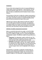
Graph for 1999 to 2006:
As we can see in this particular interval, we are able to add a line of best fit as well, thus showing that the graph is again undergoing a linear trend which can be interpreted as a linear function. The same equation would be used which is:
fx= ax+b
the two values for this particular interval would be (4, 566.7) and (6, 550.5)
Hence substituting the values:
4a+b=566.7
6a+b=550.5
Hence solving the equations using Polysimul:
Forming the final equation:
fx= -8.1x+599.1
Here is the equation of the line against the graph:
And therefore, the model that can fit the data points of the fish caught in the sea is:
fx= 26x+444 at 1980≤x≤1988
fx= 10.31x3-88.08x2+192.89x+334.53 at 1989≤x≤1998
fx= -8.1x+599.1 at 1999≤x≤2006
Plotting of points (Fish Farm)
Trends found in graph
As we can see from the graph of the fish caught in fish farms, there is a great exponential increase from years 1980 to 2000 as the graph depicts a upward sloping exponential curve. Then, from 2001 to 2002 a steep decrease is observed in the graph, followed by another upward slope from the year 2003 onwards.
The data points in this graph are much lower than that of the data points of the fish caught in the sea and as a result, the mathematical model found previously cannot be used for this set of data points. If this graph were to be plotted against the first graph, it would stay too close to the x-axis, thus not being able to utilize the model found earlier. Therefore, a new model must be suggested for this set of data points.
Suggesting new model for Fish Farm
Just as the previous graph, this graph can be described by a piecewise function, and hence this graph will also be broken into 3 intervals namely,
2004≤x≤2006
2001≤x≤2003
1980≤x≤2000
Graph for 1980 to 2000
As we can see there is an exponential trend in this graph, so it would be best interpreted by an exponential function.
Using the graphing software and the PolySimul tool on the GDC, the new equation of the graph in this particular interval is:
fx= 1.023(1.22)x
And here is the equation of the curve against the graph:
Graph for 2001 to 2003
This particular interval in the graph displays a linear trend and therefore can be satisfied with a linear function.
Using the graphing software and the PolySimul tool on the GDC, the new equation of the graph in this particular interval is:
fx= 9x+254
And here is the equation of the line against the graph:
Graph for 2004 to 2006
This interval in the graph also displays a linear trend and can also be satisfied by a linear function
Using the graphing software and the PolySimul tool on the GDC, the new equation of the graph in this particular interval is:
fx= 16x+300
And here is the equation of the line against the graph
Discussion of trends
After observing trends from both the sets of data points for the fish caught in the sea and the fish farms, we can notice that during the exponential increase of the total mass of fish from fish farms, there is a gradual decrease of the total mass of fish caught from the sea. This is how the relationship between the two different environments is brought out.
A number of causes or parameters could explain this situation between the fish from the farms and the sea, including government policies. For example, a law could be enforced by the government against sea-fishing, to promote the domestic farm fishing which lead to the exponential decrease for farm-fishing due to increase in demand for fish from the fish farm
Another cause could be weather conditions, for example a stormy weather which would be inconvenient for fishing from the sea, which will cause a slow decrease in the amount of fish caught from the sea. This would lead to an increase in demand for farm fish as the demand for sea fish was not met, hence explaining the increase in the fish farm.
Sewage dumps from large factories or industrial structures could also play an integral part in the deterioration of amounts of fish caught from the sea. As the sewage dumps pollute the sea, the amount of fish in the sea tend to decrease due to increased deaths in the sea, thereby again reducing the amount of fish caught from the sea, and in turn increasing demand from fish from the farms.
Finally, advancing technology in favour of fish farms could also be vital in the increase of fish from the fish farms, due to increased variety and improved quality from the fish in the farms, which is also another likely cause for the exponential rise of amount of fish in fish farms.
Possible Future trends
While a gradual decrease is noticed from fish from the sea, it tends to show an upward linear trend towards the end of the graph, as opposed to the continuous display of an exponential trend in the fish from the farms. Possible future trends would be a direct continuation of each of the trends from both of the environments. However, due to its exponential increase, the fish from the fish farms will catch up with the fish from the sea, and the two graphs will intersect, in turn causing the farm fish to replace the sea fish as the main supplier of fish. To determine the exact point in time in the graphs where they will intersect, the functions from the third interval from each model suggested for both data points can be equated, giving an x value of 40, which is the point in time where the two graphs will intersect, which is approximately in the year 2020. This break-even point will cause the fish from the fish farm to replace the fish from the sea as the main contributor or supplier of fish for the many years to come.