Such a graph is generally denoted by the function
Due to the visual similarities, we may judge the dependence of the female BMI on age to be such a cubic function of a polynomial to the third degree and thereby set about finding the equation that fits the graph.
To create a model that corresponds to the graph of a polynomial to the third degree, we must solve for the given function a system of four unknowns using four points from the graph and therefore four equations.
The four points chosen were:
P1 (2, 16.40) P2 (5, 15.20)
P3 (11, 17.5) P4 (16, 20.4)
When inserted into the formula, the following equations were attained:
When simplified:
➔
There are many possible ways by which to solve for the function of the graph, including the method of substitution:
Here, one variable is expressed in terms of the others then the result is substituted into the remaining equations. The resultant equations are then simplified until one variable is fully solved for. This is consequently substituted back into the remaining three equations and we move onto solving the system of equations for the next variable. This process is continued until the values of all the four variables have been determined; a situation from which we may attain the function of the curve.
Yet this process, despite being simple, is one prone to many careless mistakes due to its length. As exact values are key in this highly specific model, it is far more advisable to solve the system using a neater, shorter method:
When having two or more equations, we may solve them through the use of matrices. The availability of a GDC simplifies the process even further;
With the four equations in four unknowns, we enter them in a 4 x 5 matrix (in our case: [D]), placing the constant in the far-right column:
We then »quit« this area of the GDC, return to MATRIX, move over to the MATH menu and take choice B: rrf( , press enter, then insert the matrix name ([D]) . Upon pressing ENTER, the whole system will have been solved for you.
Yet the most appropriate way would probably be the GDC’s cubic regression option which calculates the best fitting function using the given points: from having entered those points into the STAT option under L1 and L2;
We return to the statistics menu (under STAT), go to the CALC submenu, then select CubicReg. We then enter the commands; L1, L2,Y1 and, upon pressing ENTER, attain the image below:
From the general equation of a cubic function, we have now derived that:
a=-0.0040727906, b=0.1535049941, c=-1.275202327 and that d=18.27170795, giving us the function:
As we can see, the cubic function fits among the median BMI levels of the developmental years of human female life perfectly-no variation is found. Yet, though the function is a good fit for the data that we have; the first 20 years of life, given the complexities of the human body and nature, it is rather improbable that the function should fit the whole life-span of BMI rates; especially as the function later goes on into the realms of negative numbers which do not even exist for our variables. According to this function, a median-listed woman of age 30 would have a BMI of 0kg/m2. The representation of the BMI by the function of this graph is appropriate to this small age-range but the basic extended shape of the curve of a polynomial degree would never change, regardless of the restrictions in parameter we may use upon it, hence being inappropriate to the fluctuations of the general, wider scope of the median BMI.
There are, of course, also other functions that model, well or badly, the data given.
Here are the set examples for most of them:
By the comparison of these, we may see that many fitting trend lines are possible yet our data records the changes of female BMIs in accordance with age; from toddlers to young women, where the body mass index changes quite significantly, predominantly due to the many biological changes simultaneously occurring in the body. If we look to the predictable data of the lifespan BMI of an elderly lady, we can naturally predict that, when (if) she bore children, there should be a natural rise in BMI during those periods and a slow rise throughout the mature part of her lifespan (unless particular weight-reducing measures were taken) due to the slowing down of the metabolic system and (upon average) the reduction of physical activity. Taking this into account, most of the above models are a plausible fit. We must also keep in mind that this data is merely the median-it does not tell us of any specific examples. A possible (though highly improbable) reason to the fluctuation of the curve of the graph could even be that the generations differ among themselves, having been born/raised in somewhat different circumstances. Overall, the sample of data given is far too limited to draw reliable conclusions. We are given neither any information regarding disparities nor any raw data to devise our own conclusions from, presenting many limitations to our possible conclusions.
Since our data is restricted, we must assess the part of the graphs of the functions with the same restrictions. According to this, the quartic trend line fits perfectly, with the quadratic not being too far behind, given that our data has been put to the median rather than any other form of such assessment.
The graph of the quartic function seems reasonable in that the BMI does not drop to impossible depths, yet turns so when it later reaches impossible heights. However, it is the best fit according to the given data where there is no significant variation from the median BMI.
The graph of the quadratic function is better fitting to the issue on a larger scale, if such an issue can be assessed adequately in such an investigation.
But personally, I feel that the general form of the above power function depicts the overall, long-term situation most favourably. Though the fluctuation in the BMI of your average 2-9year old is not taken into account, more moderate and believable BMIs in the later stages on life are presented. It is the model I shall use to estimate the BMI of a 30-year-old woman in the US;
y=BMI
y=12.31250011*30^0.1659723381
y=21.6524735
- The median BMI, according to the model comprised of the data given and the power function, of a 30 year old female in the US is estimated at 21.65.
This is not an overly reliable result as the model takes preference to depicting the longer term situation. Furthermore, it is based upon the data collected for mainly not-yet-fully-developed females, few of whom will have already born children and undergone other such activities that may have affected their BMIs. The case of a thirty year old woman would, however, be somewhat different. Note that the resultant BMI is equal to the median BMI of a 20 year old.
As the BMI is dependent on both a person’s weight and height, a study of the median BMI of the females of Guatemala, for example, is likely to be quite different due to the average height of a Guatemalan female being somewhat less than that of an average female in the US. The culture and very different way of life, typically involving larger quantities of festivities and hence food, may also have an impact on the average weight of women hence giving to a higher median BMI.
The data for females in 1995 was as follows:
In Due to the previously mentioned lifestyle and physical factors, we may observe that the median curve for Guatemala indicates, when compared with the US median, a lower BMI at the younger ages, then a steeper rise in body fat leading to a median of higher BMI in the later stages of the female development. Due to this specificity of backgrounds, the model of the polynomial to the third degree for the USA is not applicable in this case, however, as we are indeed all of the same species with generally very similar characteristics and not overly large amounts of variation, such a cubic function is still applicable, it need only be adapted to the data for Guatemala to attain the appropriate curve.
Bibliography:
Obesity and Overweight. World Health Organization: 2009. Available at: Cited: 07.11.2009
Exceptions where BMI may be unrelated to the probability of the said conditions due to physical deformations have been known to exist.
(the data missing is not of vital importance to the situation)Data attained from: