This model does represent our data quite accurately but as I discussed above, its limitatiations keep it from being an appropriate model for population growth. The average systematic error percentage is 1.7 %.
Now we take in account the formula that the researcher suggested which is:
, where K, L and M are parameters.
With the use of GeoGebra4 we found the approximate values for K, L and M that best fit this model.
K=2255
L=14
M=0.03
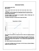
*year is shown as 50 – 1950, 70 – 1970 etc, whilst 100 represents 2000. [plotted with GeoGebra4]
We can clearly see that this function fits the model better, there are more improvements than the linear function model and it represents the data more realistically and its approach is more detailed instead of the much broader one of the previous model.
When we look at this table, we can see that the systematic error percentage is lower than the one of the linear model. The average systematic error percentage is 1.5 %.
By taking these two approaches, we are able to see the difference, evaluate and find the proper function that most likely suited the model I was given, and got the points presented with quite an accurate precision.
One of the limitations that were noticed in the first linear model function was that although it approached the points close, it wasn’t accurate enough, and it does not represent the population statistics as we would imagine, because of its tendency to portray results just in the short run. If we see at the beginning of the 1st picture of the linear function above, we can notice that the line is decreasing and eventually going towards the negative set of numbers. We know that this is not possible when it comes to the count and growth of population, so it stands out as the biggest weakness of the model I presented. Also, in the future, the line tends to grow constantly, just as it is expected from a linear function, but that would mean that the population is growing to infinity at a constant rate, and does not account for any changes that might happen, so the second biggest weakness and limitation of the first model is its ability to predict results and data.
If we take this model as the one that should be considered when looking the growth of population of China, we would find out and expect a very fast growth to several millions of people in the next couple of years, and believe that the population in the past at one point had a negative value (which is impossible to state).
With the second function we are able to come to an even more accurate model that resembles closely the original data points given, which helps us to view the model with a function that is able to cover some of the weaknesses of the first model. We can see that it does start quite realistic, rising at the present moment, with a continuous but not constant rate of growth which does seem more reliable than the constant one of the linear model.
Its limitations could be its lack of complete accuracy, or just a bigger accuracy, its possible predicaments, even if they do come very close to the data, they still do not account any possible changes to the way the population grows, but the data would be correct if the population continues to grow under the same circumstances and at the same rate as the present time in the model.
If we take this model as the one that shows us the growth of the population in China, we are left with a slightly more clear and precise model that would give us more or less close to accurate answers as to how the population was in the past, how it increased, the present time and the continuality of the growth of the population after the present
So the choice as to the more appropriate model for this particular situation would definitely be the second, logistic model because of the bigger accuracy and better predicaments and past data presentation than the linear one.
Now we take a look at the data published by the International Monetary Fund from 2008.
We can see that the data above closely resembles the first data.
*the scattered points show us a growth in population again and the values for the years are counted
as 80 for 1980, 90 for 1990 and 100 for 2000. [plotted with Microsoft Excel 2007]
As we did with the first given data on the sheet, we will start firstly with the linear equation and model.We find the slope and y-intercept and we get the following graph
Type equation here.
*[plotted on GeoGebra4]
We can see that the linear model did not work out as accurate as with the first model for the first table of data. The possibilities for that are because this has some newer data points that don’t increase with the same intensity as before. The population is still growing but not as fast as before, and this is one of the models where we can notice why it is not wise to use a linear function model to present a population growth.
With the table above we can see how the error percentage has increased significantly from the model based on the first data we had. The average systematic error percentage is 1.88%.
Now for this data I will try to model a presentation through a logistic function, or more precisely, a model based on the logistic function we were given.
The values are:Type equation here.
K = 1589
L = 37.6
M = 0.05
*[plotted with GeoGebra4]
What we are able to interpret with the graph above is that the formula fits the model quite good and accurately.
The average systematic error percentage is 1.4 % which by itself is quite good for our model, and it is represented close to its original data.
And again, as expected, the logistic model gives us a better presentation of the data given by the IMF about the population growth, because just as it was with the first data for the population, the linear function gave approximate results that make sense just at the present moment, and are quite inaccurate when we discuss about the long run of the population growth. The logistic model on the other hand, gives a more realistic approach as to the population growth and it has better accuracy than the linear model.
If we combine both data and tables we got we will get the following linear and logistic models and tables for the data:
*[plotted with Microsoft Excel 2007]
Linear model:
*[plotted with GeoGebra4]
Logistic model:
*[plotted with GeoGebra4]
Table:
The average systematic error percentage is 1.7% and considering the range of the data, this is very close to being considered as accurate data, and the precision is high.
So I can conclude that the model that I developed fits the data rather good and accurately, the linear models having their limitations in the prediction and long run data, altogether with the past impossibilities they present whilst the data for the present moment seems as though it is presented correctly. The logistic models, adjusted to the data that was given to us, best fit the overall model and presentation of the population in China because it models the data with high precision (or rather with low imprecision), and it takes into account any possible long run changes to the population, and can be described as the best-fit model to represent the data in this case.