The zeros of a derivative function correlate directly with the local minima and maxima of the corresponding polynomial because it is at the minima and maxima where the slope, or rate of change, is zero. For example, the zeros to the derivative function, f’(x), are (1,0) and (3,0). These zeros can be found by analyzing the table created for the approximate graph of the derivative function by using the equation f ‘(x)=f(x+0.001)-f(x)/0.001. Furthermore, the local minima and maxima of the polynomial occur at the same points as the zeroes of the derivative. At these local minima and maxima, the graph is no longer increasing or decreasing therefore making its slope zero. Because the graph of a derivative function corresponds directly with the polynomial’s instantaneous rate of change the derivative matches up directly with the slope of the polynomial. This is why the derivative’s zeros are located exactly where the original power function’s slope is zero: at its minima and maxima. Therefore, the zeroes of a derivative occur at the polynomial’s exact minima and maxima because this is where the polynomial’s slope is exactly zero and a derivative is simply a function of slope.
To find the function of a derivative without simply using the power rule algebra must be used in accordance with the previously calculated zeros. Because it is agreed that the zeros of f’(x) are (1,0) and (3,0), it can be concluded that the equation of the derivative must be f’(x)=k(x-1)(x-3) in which “k” is some number. To find k, a non-zero point on the derivative’s graph must be used. In following case that point will be (4,9). Therefore, after plugging in f’(x) and x, 9=k(x-1)(x-3). After solving the equation for k algebraically, k is equal to three. Now the equation of the derivative can be found by plugging the number three in for k: f’(x)=3(x-1)(x-3). Now, by using algebraic laws of distribution, a power function is derived: 3x2-12x+9. Therefore the derivative of x3+6x2+9x is 3x2-12x+9. In conclusion, by plugging in three points on the graph of a derivative function: the already calculated zeros and one random point, an equation of the derivative function can be found algebraically.
When juxtaposing the two equations f(x)= x3+6x2+9x and the derivative, f’(x)= is 3x2-12x+9, it is seen that the derivative function is to one less degree than the original polynomial. As can be seen on the graph of the polynomial function and its equation, the function as two zeros, one of which is to the degree of two, and a total of two minima/maxima. Furthermore, the graph of the derivative function as well as its corresponding equation is observed to have only one local minimum/maximum and two zeros, both of which are to the degree of one. Therefore, it is seen that the number zeros of an equation (and their degrees) are represented by the degree of the function. It is also seen that the amount of local minima/maxima are one less than the degree of the equation (or the amount of zeroes). Because the zeroes of a derivative function are based off of the corresponding minima and maxima of a polynomial, and because there is one less minimum/maximum than the amount of zeroes of a polynomial, there is one less zero in the derivative function than in the initial polynomial function. And because the degree of a function is directly based off of the amount of zeroes, a derivative function is to one less degree than the polynomial. In summary, a derivative function will always be to one less degree than the preliminary polynomial.
After factorizing a function to find the zeroes of that function, it is possible to make a conjecture about where the local minima and maxima will be located on the graph by simply using the location of the function’s zeroes. For example, if the equation g(x)=x4-3x3-24x2-28x were to be factored out completely, it would be x(x+2)2(x-7). Therefore the zeroes of the function are (-2,0), (0,0), and (7,0). Because the graph must cross the x-axis at negative two and at zero, there must be a minimum or a maximum between the two points in which the graph changes direction. The same thing is also true between zero and seven. Also, because (x+2) is to a degree of two, negative two must also be a minimum or maximum. Therefore, the three local minima/maxima of g(x)=x4-3x3-24x2-28x must be between negative two and zero, and zero and seven, and at negative two. After graphing the equation it is seen that there is, as predicted, a local minimum at negative two, a local maximum at about negative zero-point-seven, and a local minimum at about negative five. Therefore, it is possible to make fairly accurate estimates regarding the locations of minima and maxima based solely on the zeroes of a function.
The highest possible amount of local minima and maxima that a function can have depends on the degree of the function and visa versa. The number of minima and maxima in one less than the degree of the function because there is only one local minimum or maximum between every two zeroes of a function. Therefore a function to a degree of six will have a derivative function to a degree of no more than five. The original function to a degree of six can at have at most a total of five maxima and minima, meaning that the function will have a slope of zero at the most five times. Because the derivative is based off of the rate of change or slope at various points, the derivative will only have five zeroes because the initial function only comes to a slope of zero five times. And because the amount of zeroes of a function corresponds to the degree of the function, a derivative function will have a degree one less than the original function. Therefore, the derivative of a function to a degree of six has a degree of no more than five. In conclusion, the amount of minima and maxima a function can have depends on its degree, which is why a derivative function is to one less degree than the initial function.
To conclude, a power function’s zeros are based directly off of the degree of the equation, and the total number of local maxima and minima of the equation is one less than the degree of the equation because for every two zeros there is only one maximum or minimum. Furthermore, because a derivative function is based off of the slope of the initial polynomial, the polynomial’s minima and maxima and the derivative function’s zeros. Therefore, the derivative function is to a degree of no more than one less the degree of the original polynomial. A general equation can therefore be created to find the derivative function for any polynomial function to a degree of n: if a polynomial function is represented by axn+an-1xn-1+…+a2x2+ax+a, then the derivative of that function is represented as: nanxn-1+(n-1)an-1xn-2+…+2a2x+a1. This equation could therefore be used to find the instantaneous rate of change for any polynomial function at any given point and could be used to track population changes or other data based off of polynomial functions.