It is important to remember the assumptions we are making here. In real play it is unlikely that a player’s point probability would remain constant throughout play. We have not taken into account factors such as tiredness, confidence etc. which would seriously affect the game. With these caveats in mind, however, we can use the model to predict what might happen in an actual game.
Short game play:
Using the same players A and B from above, we may imagine a version of the tennis rules in which to win a player must have above four points (as the usual rules go) but in which, if both players have three points, deuce is called and the next point determines the winner. This scenario means that no game may go beyond 7 points.
We can model games as arrangements of 4 A’s and 4 B’s in 7 spaces, thus:
Number of possible games
Some of these games finish earlier than 7 points, however. For instance, the arrangement ‘AAAABBB’ would finish at 4 points, with the score 4-0. We can therefore subtract such instances to work out the number of games of exactly y points.
y=4:
y=5:
y=6:
y=7:
Note that each of these numbers represents the number of games of exactly y points, with either A or B winning. Half of these represent A winning, and half represent B winning. We can hence work out the probability of the game lasting y points, where n is the number of games of that point length:
This can be shown as a histogram:
Based on this data we can calculate the probability that A wins the game:
The odds that A wins are therefore:
For more general players C and D with point probabilities c and d, the probability that C wins is given by:
Note that because on one point C and D’s probabilities of scoring are mutually exclusive and exhaustive, we can say that:
In this way the probability of C winning can be written entirely in terms of C’s probability.
Longer game play:
In the above examples the rules ensured that y, the number of points played, could not exceed 7. If instead the rules become that to win, a player must have 4 points and be 2 points ahead of their opponent, we can produce theoretically infinite games. The word ‘deuce’ will be used to refer to a state where the scores are equal and greater than 2, and the word ‘advantage’ will refer to the state after deuce where there is a 1 point difference.
To model this situation, we can consider two possibilities: a game with deuce and a game without deuce. We will discuss the latter first.
If the game is to occur without deuce, it must end at 4-0, 4-1, 4-2, or the reverses of these. Any other score would either be too low to win, or would have involved deuce (e.g. a score of 4-3 could only occur after a score or 4-2, which is already accounted for, or 3-3, which is deuce). The probability of each score can be calculated as follows:
We can use a similar calculation to find A’s chance of winning in a non-deuce game:
We must also consider a game in which deuce occurs. After deuce, the next point brings the game into advantage either for A or for B. The point after than either ends the game or returns to deuce. For A to win he must score twice after deuce, for B to win he must score twice, and for the game to return to deuce each player must score once.
Two points after deuce, the probabilities are therefore as follows:
Two points after that, the probabilities are multiplied by (because deuce must have occurred again, and so on. The probability of A winning 2z points after deuce is first called is given by:
The probabilities form a geometric sequence with first term and common ratio . Because we know it is a convergent sequence, and we can calculate its sum to infinity:
Therefore A’s probability of winning once deuce is called become over a long game. To calculate A’s probability of winning in a game with deuce we must calculate the probability of the original deuce occurring. The score for this must be 3-3, so the probability is:
The probability of winning in a game with deuce is thus:
A’s probability of winning overall is the sum of his probabilities with and without deuce:
A and B winning are mutually exclusive and exhaustive, so they sum to 1. The odds of A winning are therefore:
It can be seen that A’s odds of 2:1 on a single point give a much greater advantage over extended play, as he now has odds of winning of almost 6:1.
We can model these probabilities more generally again for players C and D with point probabilities c and d respectively. In a game without deuce:
The probability of deuce occurring to begin with is:
Once deuce has occurred, the probability of C winning is given by the sum to infinity as above (note that must hold; the below equation fails if C is certain to score) :
The probability of C winning the game is therefore:
The odds can be calculated as:
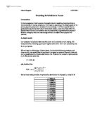
The probability distribution for C winning can be calculated for any value of c:
The relationship can be shown graphically:
This shows that when the point probabilities are close to each other (i.e. near 0.5) a small change can make a large difference in the overall game probabilities, whereas if the point probabilities are far apart a change will not make much difference.
In practical terms, this means (perhaps unsurprisingly) that matches with closely-matched players are the most exciting to watch, because a small change in the player’s relative performance can change the likelihoods dramatically, making the game less predictable.
Conclusions:
These results must be interpreted based on the limitations identified at the start. The results hold for cases with perfectly consistent players, but this is not the case in real life. The changes in performance that would result from tiredness as the game goes on, or from confidence (or the lack thereof) as one player succeeds and the other does not, would significantly change the probabilities in ways that this model cannot predict. Because of this the model would need to be made much more complex if it were to serve as a predictor of real-life situations. However, as a tool to explore the mechanisms at play in a game of tennis, the simple model that we have developed shows clearly how the players’ relative strengths affect the overall result, and also how the rules of play that allow a game to go on longer significantly enhance a strong player’s advantage, so the model is not entirely useless.