Therefore here I will add all the above fractions:
=
= 1
As the fractions sum up to 1, the values are true.
From the above values, a histogram is created using Microsoft Excel and then exported to Microsoft Word:
According to the histogram above, the modal value is 7 due to its highest probability. It would not be likely for Adam to get more than 8 points and less than 4 points by looking at the histogram above. Now using the binomial distribution, we can calculate the expected value and the standard distribution:
Expected value = E (x) = np
= 10
≈6.667
Variance =
2 = np (1-p)
=
(1 -
) =
Therefore, Standard Deviation =
=
1.4907
It is necessary to keep in mind the assumptions we have made over here. In the real game, there are many factors that influence the winning of an individual in the game, such as confidence, injury, stamina, etc., which would affect the game, and so player’s point probability doesn’t remain even. With these stipulations in mind, however, we can use the model to predict what may happen in a real game.
Part 2:
Now we look at the Non-extended game where to win, the player has to win at least 4 points and by at least 2 points. And the important part is that no game can go beyond 7 points. This means that if there is a deuce due to each player having 3 points then the following point will determine the winner of the game.
We can represent games as measures of 4 A’s and 4 B in 7 spaces, thus:
Number of games possible =
= 70
However, some of these games may finish before 7 points. We can then subtract such cases to come up with the number of games of exactly y points.
y = 4: 2
= 2
y = 5: 2
– 2 = 8
y = 6: 2
– 2 – 8 = 20
y = 7: 2
– 2 – 8 – 20 = 40
Therefore from this it can be seen that there are (2 + 8 + 20 + 40) = 70 different possible ways in which the game can be played showing the different combinations possible when a player loses all the games. After finding the different ways the game can be played in, now I shall work out the probability of Adam winning the game. The different possible ways in which Adam can win the game are 4-0, 4-1, 4-2 and 4-3; and so now I will have to find the sum of probability of these events taking place.
The model for the probability of a particular outcome of Adam winning the game would be:
P (X=3) =
The part of the equation inside the brackets is the last point and this part of the model has no variables because it is the last point and should always be won by Adam.
Below are the ways in which Adam can win:
Therefore the probability of Adam winning the game is the sum of the above probabilities:
Hence the total probability =
=
The formula for the odds of Adam winning=
The probability of Adam winning was calculated above and the probability of him losing will be (1 – probability of Adam winning). Therefore the odds of Adam winning the game:
=
=
4.77
Therefore the odds of Adam winning are 4.77:1
Now to generalize the equation so that it can be used for any other players with different probabilities, we just have to substitute the probabilities of their success and failure in place of
and
. Here we shall be using variables c and d in place of the probabilities.
Now the probability of a Player C winning will be the same as that of Adam, i.e., the possible ways of winning would be 4-0, 4-1, 4-2 and 4-3 and the winning/ last point will be fixed in each game.
Therefore the probability of Player C winning the game would be:
= c4 + 4c4d + 10c4d2 + 20c4d3
As on one point C and D’s probabilities of scoring are mutually exclusive and extensive, we can say that:
c + d = 1
Therefore, d = 1 – c
In this way the probability of C winning can be written completely in terms of C’s probability.
Part 3:
In the above part, the rules said that y, the number of points played, couldn’t go beyond 7. But according to the question, to win the game, a player must have 4 points and be 2 points to the lead of their opponent and so we can hypothetically generate countless games as the player could keep winning one point each and keep getting back to deuce.
To model this situation, I will consider two possibilities: A game without deuce and a game with deuce. I will discuss the former one first.
A Non-Deuce Game:
The possible outcomes of a non-deuce game are 4-0, 4-1 and 4-2.
The probability of Adam winning a non-deuce game can be found out by the equation used before:
P (X=3) =
=
=
Therefore, probability of Adam winning a non-deuce game =
A Deuce Game:
Now I will look at the possibility of Adam winning a deuce game. The deuce will take place when the score is 3-3. The next point after deuce will bring advantage for either one of the players. The game will only end if anyone player scores two consecutive points after deuce or else the game will return to deuce again. Therefore the probability of a deuce occurring during the game:
P (X=3) =
=
From this value, a definite fraction Adam wins and the other Ben wins. So now I will calculate the fraction of Adam winning a deuce game, which I will add to the probability of him winning a non-deuce game to deduce the odds of him winning.
After the deuce, for Adam to win the game, he will have to win two consecutive points and the probability of that will be:
=
Now the probability of both scoring one point each after the deuce and therefore again having a deuce:
=
The infinite geometric series goes on as Adam would have to win 2 consecutive points and the deuce can go repeatedly, therefore the total of infinite geometric series should be calculated. Its formula is:
Su =
[Here a is the first term of the series and r is the ratio]
S =
=
Therefore the probability of Adam winning a deuced game =
=
To find the total probability of Adam winning the game, I will add the probability of him winning the deuce game and the non-deuce game.
Therefore, the probability of Adam winning the game =
=
Probability of Adam losing the game = 1 -
=
Therefore the odds of Adam winning the game =
= 5.94
6
Therefore the odds of Adam winning the game is 6:1
Now I will generalize this model so that I can find the probability of any player C’s to win a point c and any player D’s to win a point d.
The probability of player C winning a non-deuce game can be calculated using the formula:
=c4 + 4c4d + 10c4d2
The probability of a deuce during the game is calculated using the formula:
P (X=3) =
= 20c4d3
Therefore the probability of player C winning during a deuce game:
= 20c4d3
[Here
is the sum of the infinite geometric .
series where the game could go on forever]
Therefore after simplification, it is found that the probability of player C winning a deuce game =
Therefore the formula for calculating the probability of player C winning a game is the sum of player C winning a deuce game and a non-deuce game:
Therefore, P (Cwins) =c4 + 4c4d + 10c4d2 +
Therefore, the odds of player C winning can be calculated by using:
Odds =
Several values of c are substituted in the formula to obtain the probability and all the odds. Through this a pattern can be noticed which is very important and significant. As d = 1 – c was shown in the previous part, the value of d is also substituted.
Below is the table for the values of c:
From the above table it is seen that as the value of c increases, the probability of player C winning the game also increases and the odds increase rapidly, for instance, the odds during c = 0.10 is 0.001449 while for c = 0.90, the odds of winning is 690.084312; this shows that there is a huge increase. As the values of P (Cwins) get closer to 1, the odds of winning grow rapidly and exponentially. Also when the value of c is less, the odds of winning are asymptotic to the x-axis and very close to zero.
Conclusion:
The use of probability has helped to make successful assumptions and predictions in many areas such as predicting the weather, the market, gambling, etc. Probability helps us make better decisions and hence the risk factor decreases when a particular decision is supported with probability. If we look at this portfolio, it is seen that I was successfully able to calculate the probability of Adam winning the games with slight variations. Though these predictions are not always right, they give us a fair idea of what the outcome might be. The values I found wouldn’t be true and applicable all the times with different people but still give us more knowledge of the results.
There are also several limitations to my models due to which they are not entirely realistic. The point probabilities, which were given, are never constant in a real game and are influenced by many factors such as the climatic conditions, stamina of the players, injuries, etc., due to which the probability values can sometimes go entirely wrong. Even when we look at the extended game, the possibility of the game going on forever decreases the reliability on the point probabilities. But if we look on the other hand, the models that I have developed shows that how the player’s dominance over the game affect the overall results and also how the variations in the game, like changing the rules increase the possibility of a stronger player to win the game. Therefore this model is also useful to a large extent.