-
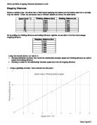
Find m (the gradient) using the following equation:
-
b is the y intercept but as the graph passes through the origin this value is 0 because while the car is moving at 0 kmh-1 the braking distance is 0 m.
-
The final linear equation is for the domain 32<x<112 because we do not know how long the thinking distance will be for any higher speeds. We could guess from the graph but in a real life situation this would be putting the drivers’ life at risk.
Although finding the equation of straight line is relatively easy, one should further prove that the line fits. Below is a table showing the original values for thinking distance and the output values from the equation, .
This shows that the line, , fits exactly with the values given.
Figure 2 has a graph with an increasing gradient and looks like a part of a quadratic curve suggesting that the braking distance increases with speed. The equation of the curve above almost follows the curve, . This can be found using a graphic calculator.
To see how well the curve fits mathematically, below is a table showing the output values from the equation and comparing them to the values already given.
We can see from looking at the table that the output values lie very close to the original values so it can be concluded that the equation is for the domain 32<x<112.
However, from a critical point of view, the values for when and are slightly further from the original values.
Figure 3
Figure 3 is a graph representing the relationship between speed and the overall stopping distance. This again is a quadratic curve and the best fitting equation (found using a GDC) is:
. This function is similar to that of figure two as both graphs show an increase and both could be parts of a quadratic curve. The main similarity between figure 1 and figure 3 is that both graphs have a positive increase.
Below is a table comparing the overall stopping distance values (obtained from adding thinking distance and braking distance values together) and the output values from the equation,
.
This function obviously does not fit as well as the last two functions although the values do link, just not very closely. If the function is changed, it may fit the top end of the x values but not the bottom, or vice versa.
The overall stopping distances for other speeds are shown below:
The graph above shows the values for the different overall stopping distances. The points in the red show the values from the last table and the points in blue show the values that were obtained from adding the initial thinking and braking distance values.
The table below shows how the new values for the stopping distance fits into the equation
The first and last values to do not fit the curve well but the middle 2 values do. From looking at the graph above we can see that all the overall stopping values sit on a curve so it is evident that the problem is in the curve function itself.