then and = 0.1875
We can present the above mentioned result as a result of the following equation:
y - y1 = m(x - x1)
So for the chosen points (64, 12) and (96, 18) the equation has the following view:
y - 12 = (x - 64)
y = x, where x is the thinking distance, and y is the speed.
So we may deduce that there is a simple linear relationship from the type:
y = ax + b, where a = 0.1875, and b = 0.
Linear Relationship
Hand calculated model
y = mx + c
(64, 12) 12 = 64m + c
(96,18) 18 = 96m + c
We consider it as a system of equations and solve it by substitution.
Substitution
c = 12 – 64m
18 = 96m + 12 – 64m
18-12 = 96m – 64m
6 = 32m
m = 0.1875
So, if m = 0.1875 then:
c = 12 – 64m
c = 12 – 64 x 0.1875
c = 0
Therefore the hand calculated model of the relationship between the speed of the vehicle to the thinking distance is y = 0.1875x
Excel Calculated
y = ax + b, a = 0.1875, b =0
Description
In chart 1, the points plotted are clearly in a straight line. This reveals the linear relationship between the points. Below we have hand calculated the equation of a linear relationship, which results in the equation to be y = 0.1875x. We use the same graphing software to calculate the equation of the line by entering the points in to the program. The program produces the same result. Both graphs overlap so only one line is visible. It is obvious that there is a linear relationship between the speed of a vehicle and the thinking distance.
Speed vs. Braking distance
Excel models
For speed vs. braking distance, the formula for a linear equation through (48,14) and (96,55) is found by:
The equation is found by y - y1 = m(x - x1)
y – 14 = (x – 48)
y - 14 = x - 41
y = x - 27 (x = braking distance & y = speed)
y = 0.8541x – 27
Quadratic Relationship
From chart two it is clear that the points represent a curve which is suitable for quadratic or cubic equation. For the quadratic equation of the type: y = ax2 + bx + c, the graphic software calculates the relationship in the following way: y = 0.0061x2 – 0.0232x + 0.6
Cubic Relationship
y = ax3 + bx2 + cx + d
The software calculates for the quadratic relationship:
a = 1.1118 – 6; b = 0.0059; c = 1.4724 – 4; d =3.0093 – 6
Description
In the graphs above, the plotted points are in a curve. This is possible in two cases: if there is a quadratic relationship or a cubic relationship. As it’s seen from the equation for the quadratic and cubic relationships, they both fit the data properly. However, the cubic function is only suitable for this data, because cubic functions go to infinity and in real terms a car is not able to go faster than a certain speed. Therefore, the quadratic relationship is more suited to the data. It also makes sense that it is a quadratic as you can only imagine as the speed is higher, the brake will be pressed down on more abruptly, therefore making the distance shorter, yet in quicker time – this justifies the quick shoot up of the line.
Speed vs. Overall Stopping Distance
Excel model
These points are not perfectly linear, so a quadratic equation might be a better fit to the points. A linear equation would be exact for the 2 points used to find the equation, but would have some amount of error for other points.
Quadratic Relationship
y = ax2 + bx + c
The software calculates for the quadratic relationship:
y = 0.0061x2 + 0.1643x + 0.6003
Description
We model only a quadratic function here, as it is justified from the last graph (speed vs. braking distance). This graph is very similar to the one of the breaking distance. It also makes sense seeing that the faster the car will be going, the time it will take to stop will increase more rapidly than the distance it takes.
Relationship between speed and overall stopping distances
Description
The clearest relation between the two models is the fact that the gradient is exactly the same on both models. It makes sense that the thinking distance curve is less steep than the stopping distance as the breaking distance is not added to the thinking distance. This graph can be used to tell how significant the braking distance is as it clearly shows the difference between the stopping distance and the thinking distance.
Additional data – Model fit
If two of the previous equations are added together /the linear equations for thinking and braking distances/, the new combined equation is y = x + x – 27 or y = x - 27
This linear equation is reasonable in the center of the domain but loses its effectiveness as distances are shorter or very large.
To get a better equation, we will use 3 of the points to find a quadratic equation fitting these points. If we use the points (48,23), (80,53), and (112,96) in the quadratic equation
ax² + bx + c = y, we get:
ax² + bx + c = y
a(48)² + b(48) + c = 23
a(80)² + b(80) + c = 53
a(112)² + b(112) + c = 96
2304a + 48b + c = 23
6400a + 80b + c = 53
12544a + 112b + c = 96
Solving this system of equations on a graphing calculator using the command rref([A]) gives the following approximate values:
[1...0...0__0.006]
[0...1...0__0.125]
[0...0...1__2.375]
respectively for the three above mentioned equations.
This is the equation y =0.006x² + 0.125x + 2.375 which will fit more closely to all of the points. It also eliminates the problem of having negative braking distances for lower speeds. This graph also increases more at the upper end to more closely match total braking distances for faster speeds.
The linear equation y = x – 27 gives a totally impossible negative stopping distance for the answer for a speed of 10 km/h. The quadratic equation y = 0.006x² + 0.125x + 2.375 gives a more reasonable answer of 4.225.
For a speed of 40 km/h, the quadratic equation y = 0.006x² +0 .125x + 2.375 gives a very close answer of 16.975.
For a speed of 90 km/h, the quadratic equation y = 0.006x² +0 .125x + 2.375 gives a close answer
of 62.225.
For a speed of 160 km/h, the quadratic equation y = 0.006x² +0 .125x + 2.375 gives a close answer of 175.98 while the linear equation gives an answer far of that.
Clearly, the quadratic equation is a better predictor of the total stopping distances.
How does it fit the model and what modifications can be made?
The additional points have been plotted in bold in collaboration with the stopping distance data created from the initial data. As we can see on the graph, the additional information is fairly accurate, and fits the model perfectly. There are no major modifications needed, as the data seems to fit on to the line rather perfectly. One minor addition rather that modification that could be made is to try the vehicle’s highest speed to see whether or not this model is valid through all the speed of the vehicle.
Conclusion
In conclusion, it is clear that there is a linear relationship between the speed and thinking distance, whilst there is a quadratic relationship between the speed and breaking and the stopping distances. This seem to be an obvious outcome because it makes sense that when the car is at a low speed, the break will be pushed down in a controlled manner, hence making the distance increase quicker than the time, where as, if the vehicle is going at a much quicker speed, the driver will tend to push down on the brake more abruptly and will stop over a smaller distance but quicker.