a≈97.087 (This value will be utilized in finding the averaged a value.)
I will complete another demonstration now using the data from year 11 which has the population of 112.8 (thousand) with the use of my GDC. The problem will be set up as follows: 112.8=a(1.03)11.
a≈81.489
When I continued this method of calculation with my GDC for the rest of the data I found the following answers in the data table below. I rounded each a value to the nearest thousandth place.
Finally, I’ll find the average of these a values using my GDC.
Rounding these values to the nearest hundredth place results in a≈76.06.
Therefore, the population model of Swaziland is y=76.06(1.03)x, where x is equal to the years starting with 1911 as the first year and y equals the population of that year in thousands. In comparison to the data, I believe this model fits fairly well. When I created a graphical model of the actual population data and compared and contrasted it with the graph of my model, I observed a pretty close relation in the trend and pattern. I made this graph with my GDC shown below.
(The square dots represent a scatter plot of the population data, and the curved line represents the graph of my model)
I am now going to use this model to predict future populations of this country. I will then compare these predictions to ones I will find from other sources and observe how reliable my model is. The years I will be using are the following: 2010, 2020, and 2030.The way I simplified the other year values will be applied to these, thus, 2010 will now be represented by 100, 2020 as 110, and 2030 as 120. In order to find these predictions I will plug the expressive year values in for x in my population model, y=76.06(1.03)x which will then give me the possible population for that year in thousands. I will implement these calculations using my GDC.
If x=100 then y≈1461.769 (thousand). Thus, the projected population of Swaziland in 2010 is 1,461,769 people.
If x=110 then y≈1964.496 (thousand). Therefore, the possible population of Swaziland in 2020 is 1,964,496 people.
If x=120 then y≈2640.118 (thousand). Thus, the estimated population of Swaziland in 2030 is 2,640,118 people.
According to the CIA Factbook , the estimated 2009 population is expected to be 1,123,913 people. Compared to my prediction of the year 2010 having the population 1,461,769 people and having the record of 2005 having the population approximately 1,317,000 people, this estimation can elicit a conclusion that the population of Swaziland is actually shrinking instead of growing as my population model portends. This shrinking could be a result of disease such as AIDS, or other environmental conditions.
I am now going to proceed in finding a population model for Japan using the same methods and ideas I did for Swaziland. I will again use the exponential function, , and find each variable using algebraic processes. The following table shows approximate populations measured in millions of given years.
I reused the same idea of simplifying the years that I did when finding the model for Swaziland. I started with 1900 as the first year, 1910 as the eleventh, 1920 as the twenty-first, and so on. These simplified values will express my x value and the years (in millions) will express my y values. I placed these values in the table below.
I am going to repeat the same procedures I used to find the model for Swaziland in finding the model for Japan. Therefore, I will first find the rate, b. To reiterate what I did in finding this value for Swaziland, I took the change in population divided by the change in year. I then added that quotient to the smaller of the two populations and divided that sum by the same smaller population. I will repeat this process using every group of two consecutive populations and their respective year. I will then average these answers to find the value that will replace the a in the model.
I will proceed using my GDC. My first demonstration will use the population 43.8 and 49.6, and the change in years is 10.
The approximate rate of change between year 1900 and 1910 is 1.01.
I will only exhibit one more example of this process, using the data from years 1920 and 1930.
Therefore, the approximate rate of change between these two years is 1.01.
By completing this process for the rest of the data, I obtained the following values that I placed in the table below. I rounded each approximate rate of change to the nearest hundredth place.
Now I’ll find the average approximate rate of change using my GDC.
By rounding this averaged value to the nearest hundredth place, I can say that my population model of Japan to this point is.
In the same way I found my a value for the model of Swaziland I will use for my model of Japan. I will plug in each set of values from the original table into the x and y places of my model thus far,, and algebraically solve for a. After finding each individual a value for each set of data I will again carry out the process of averaging to find a value that will replace a in the population model. As already stated I will be using the population measured in millions for my y values and their simplified year values as my x. I will display an example of this algebraic process below.
For the example I will be using the data from year 1, which has the population of 43.8 (million).
a≈43.366 (This will be used in finding the averaged a value.)
To find the remaining individual a values I will be using my GDC. I will only show one example of how this will be done below. For this example I will be using the data from the year 11. The set up for this example is 49.6=a(1.01)11.
a≈44.458
After continuing this process of calculating individual a values with my GDC for the rest of the data, I found the following answers I placed in the data table below. I rounded each a value to the nearest thousandth place.
I will now average all the a values using my GDC.
I will round this value to the nearest hundredth place which it will then be substituted for the a value in my population model of Japan. Therefore, the population model is.
This model fits reasonably well with the data; however, the data seems to have reached a point of leveling off as the model continues on. I have come to this conclusion by studying the graph I made on my GDC.
The square dots represent the data from the table and the curved line represents the graph of the model I made. As you can see the pattern of the scatter plot appears to be leveling off while the curve continues.
Even though I do not think my model would be the best choice to predict future populations, I am going to utilize it in finding estimated populations of the years 2010, 2020, and 2030. I will go ahead and simplify these year values like I did with the other data, consequently, 2010 will be represented by 111, 2020 by 121, and 2030 by 131. I will then compare these estimations with predictions from other sources to examine the reliability of my model. In order to predict these estimations I will plug the simplified year values in for x in my population model, y=47.82(1.01)x which will then give me the possible population for that year in millions. I will accomplish this using my GDC.
If x=111 then y≈144.305. I can, therefore, say that the estimated population of year 2010 in Japan will be 144,305,000 people.
If x=121 then y≈159.403. Hence, the estimated population of Japan in 2020 is 159,403,000 people.
If x=131 then y≈176.080. Thus, the population of Japan in 2030 is estimated to be 176,080,000 people.
According to the CIA Factbook, , the estimated population of Japan in July 2009 is 127,080,000. In comparison to the estimated population in 2005, my conjecture of the population leveling off seems to be true. The CIA Factbook states that the estimated population growth in 2009 is in fact a decrease of -.191%. This decrease is consistent with my observation of the leveling off in the graph. This percent decrease in population could be due to the idea that Japan’s population has reached its capacity, or disease and other economical issues could be the cause.
The Verhulst-Pearl Model might be a better function to depict the relationship between years and population of Japan than the exponential one I created. This model is a logistic function that could represent my conclusion of the data leveling off, because this model contains a capacity, or limit. This means that the graph will reach a kind of peak and level off. The Verhulst-Pearl Model is the following:, where t is time, measured in years after 1900, and is the population, measured in millions, at time t. k is approximately constant. is the population in 1900 and M is the limiting population (in millions) which may be considered to be the maximum population capacity of the country could support under given social and environmental conditions. I am going to assume that M=150.
Due to what I already stated about P0 being the population in 1900, since I am using 1900 as my initial starting year, I can conclude 1910 as being the tenth year, 1920 as the twentieth, etc. This also enables me to declare that P0 = 43.8. I can now plug everything I know into the Verhulst-Pearl Model. Since I know M=150, and P0 = 43.8, I can rewrite the model, as the following:
This is capable of being simplified even further to.
If I take known values from the data table and place them into their appropriate places in this function, the only unknown variable will be k, the constant. This value can be solved for algebraically in order for this function to be utilized in finding either population or year of its corresponding time or population. In this portfolio I will be using this model to find a more valid prediction of the population of Japan in 2010, 2020, and 2030.
I am going to find this constant by means of inserting the years from the data table in for the t variable and its respective population for the P(t) variable. I will do this for every set of data with the exclusion of the initial year, and then I’ll average the individual k values. The exclusion is due to the fact that k would be impossible to calculate, since the variable t would be equal to zero. To start with, I’ll display a revised data table that will show how I simplified the year values for this model.
I am now going to demonstrate how I am going to algebraically step by step solve for k. I arbitrarily chose to use the data from year 50. Therefore, P(t)=83.2 and t=50.
Therefore, by replacing these variables, the equation can be shown as .
First, I will cross multiply to eliminate the fraction. Then I will use the distributive property and other algebraic operations to simplify. I also will be utilizing logarithmic properties.
–k= -0.0221046912
k≈0.022
I will now repeat this process for the rest of the sets of data in a more efficient way with the use of my GDC. I will demonstrate one of these calculations below using the data from year 10.
Therefore, for this set of data, k≈0.004.
By proceeding to calculate these individual k values for every set of data except for the initial year, I found the following values placed in the data table below. This table is to delineate what t and P(t) I used in the function obtain each value. I rounded each value to its hundred thousandth place
I will now average all of these individual k values using my GDC.
Therefore k≈0.024.
Thus, the Verhulst-Pearl Model for Japan according to my calculations is . I am now able to use this function to find a probable population for the years 2010, 2020, and 2030. I will do this by first simplifying the years in proportional values consistent with the simplification I applied to the years in my original data table for the population of Japan. Therefore, 2010 can be now represented by 110, 2020 by 120, and 2030 by 130. Then I will perform a calculation for each by simply replacing the t value with one of these year values and solving with my GDC. These calculations are shown below.
If t=110 then P(t)≈128.490. In other words, the estimated population of Japan in 2010 is about 128,490,000.
If t=120 then P(t)≈132.591Therefore, the population of Japan in 2020 is predicted to be approximately 132,591,000.
If t=130 then P(t)≈135.996. Thus, in 2030 the population of Japan is expected to be near 135,996,000.
I think these predictions are more probable. They fit with the trend of the data more closely, as could be observed by the graph I made with my GDC.
The last three points on this graph are data predicted from my model. As can be observed, the graph of the model follows the pattern of the seeming “leveling off”. This results in the predictions being more feasible.
These estimates fit better with the projections from CIA Factbook, which stated that the estimate 2009 population would be 127,078,679. Compared to the 2010 projections from my model, it is fairly close. I believe this form of model is more preferable because of its having a capacity, which I had mentioned earlier as a possible part of the reason Japan’s population appears to be leveling off.
Another way I can check for accuracy of predictability in this model would be to use it to calculate population estimates for past years and compare them to the actual recorded populations. I will demonstrate this below using my GDC with year 30.
As listed in earlier pages, the actual population in year 30 was about 64.5 million. According to my model, the population should be approximately 69.1 million. As you can see, the population values are similar but not equivalent. This is a representation of how accurate is my model’s ability to predict. Although it is not a perfect model, it is able to calculate reasonable results that can assist in population estimates. Overall, I think the logistic model is a better fit for determining estimations of future populations.
Works Cited
“Japan.” CIA - The World Factbook. 23 Apr. 2009. 13 May 2009 <https://www.cia.gov/library/publications/the-world-factbook/geos/ja.html>.
“Swaziland.” CIA - The World Factbook. 23 Apr. 2009. 13 May 2009 <https://www.cia.gov/library/publications/the-world-factbook/geos/wz.html>.


