Diagram
Method
The experiment was done through the following steps:
- The object ‘x’ was weighed on an electronic balance
- The diameter and height of the object was measure if the object is a cylinder and the length width and height of the object was measured if the object is rectangular.
- The lengths where measured with a Vernier callipers
There are six different objects
Results
The relationship between Mass and Volume is proportional as we can see from the formula stated below:
D = M/V
Where D is the density
M is the mass
V is the volume
We can rearrange the formula to enable us to draw a direct proportionality graph like this
M = DV
y = mx
where Mass is on the y axes and volume on the x axes and the gradient would be the density.
The gradient on graph 1 is 8.4, this means that the density of the material is 8.4gcm-3.
In this graph there are two outliers; object E and F. Object E is an outlier because its volume was not measured correctly, it was of cylindrical shape with a small hook on it and the volume of hook was ignored since it was hard to calculate. The calculated density of object E is 8.5 gcm-3. Object F was an extra material that we tested and we assumed that is was of the same material as the rest of the objects, however the graph clearly shows that this is not the case, its position is far off the line of best fit with a calculated density of 7.7 gcm-3.
Extreme lines could not be drawn on this graph because error bars could not be drawn on the first three values since the uncertainty was negligible, however the values that did have large enough uncertainties did not come in contact with the line of best fit.
To try to be able to draw extreme lines, I drew another graph ( graph 2 ) where I tried to manipulate the line of best fit such that object E which has an error would be in contact with the line of best fit.
From the graph 2, the calculated density is 8.45 rounded up to 8.5 +- 0.3 gcm-3. This is of course an inaccurate value since the line of best fit went through an object of which the measurement of volume taken was less than it should have been giving us a larger value for density ( since volume and density are inversely proportional ). From this information I calculated the actual volume of Object E which is 8.1 cm3 ( calculations and justification shown in the calculations section). The uncertainty obtained from graph 2 is what we need, thus we can write the density as;
8.4 +- 0.3 gcm-3
Conclusion
From this experiment I can conclude
The density of the materials used is 8.4 +- 0.3 gcm-3 according to literature, there are three metals that have this density, they are; brass, electrum and silver nickel. Both silver nickel and brass are of a shiny silver colour and the metals I tested where not shiny silver, therefore the metal is brass.
Evaluation
From this experiment I can evaluate the following
- The volume of object E was not measured accurately which could clearly be seen on the graph
- The density alone does not give us a certain answer to identifying the metal since a couple of metals have the same density as brass.
- The volume of the objects measured could have been measured with a higher precision
To improve these weaknesses we could
- Measure the volume of the hook on object E using a string for the height and a Vernier callipers for the diameter
- Measure the melting point of the metal which will give us a more certain answer to which metal the objects are.
- Measure the dimensions of the object with a screw gauge which has a much lower uncertainty, this will obtain more precise results