Processed data – Table of Processed data
Graph of processed data
Processing Data
1. Q = mLf This is the equation to find the energy required to melt 28.50g of ice at 0°C where ‘m’ is mass of ice molten; Q the energy supplied by the electric heater; Lf is the latent heat of fusion of the ice.
2. Rearranging the formula in terms of Lf.
3. “The electrical energy supplied to the heat in time‘t’ is equal to V I t where V is the p.d. across the heater, I the current through it and t the time it has been operating for.”
Q = VIt
4. Merging equations 2 and 3 we get a new formula to find the latent heat of fusion of ice.
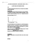
5. From the graph it is possible to take the gradient which is mass per seconds. However, the inverse of the gradient will be seconds per mass which will be a portion on the equation in equation 4.
6. =>
=>
=>
=>
= 648.6117433 J
650 Jg-1
Conclusion
In this experiment, the latent heat of fusion of ice was investigated. By the results, it is accounted that the latent heat of fusion of ice is 650Jg-1.
It was possible to draw a best fit line which accounted that the average mass melted and the time that the ice took to melt that in its turn did not pass through the origin. Moreover, the best fit line does not touch many of the error bars. Taking into account the two latter statements, I would conclude that the time taken for the ice to melt and the average mass of molten ice are not linear i.e. quantities are not directly proportional.
Evaluation
The graph above shows that the results tend to be linear. This assumption is taken by looking at the line of best fit. Though, it does not pass through the origin due to errors. There were some systematic errors as well as random errors.
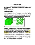
There were some systematic errors as from the stopwatch. Though this error was constant during the whole performance of the experiment, it still did not affect much. On the other hand there were also some random errors. As I was melting the ice with the electric heater, I did not push the ice towards the ice. This caused the ice on to melt entirely by the electric heater at the bottom of the funnel, where the ice was pulled automatically by the pressure of the ice above.
If we look at the graph, the error bars are not consistently the same size. However overall, they are not very big, suggesting that the random errors though controlled to some extent, still act slightly during the experiment. Evidence for systematic error would be that the graph does not pass through the origin. Due to the fault in the apparatus used, the y-intercept that should have been through the origin has been shifted.
Improvement
The random errors should be looked closely at this experiment. I noticed that I was not consistent in melting the ice. By this I mean that I should have paid close attention when pulling the ice towards the heater. With this done, the amount of ice molten at the top of the funnel would have been the same as the ice molten at the bottom of the funnel keep the melting process consistent.
The apparatus used such as ammeter, voltmeter and stopwatch contributed immensely towards the systematic error. Though, out of the 3 apparatus mentioned above, the stopwatch contributed the most to this part of the error. I would suggest that the ± 2 would be due to my reaction when stopping the stopwatch. To avoid this type of error I would use the IT system available so that the time at which the experiment should stop is kept constant.
It is worthwhile considering also the voltmeter and the ammeter. This two apparatus are limited to ± 0.5 and ± 0.1 accordingly. It clear that this was a very small error and that would not have affected much the outcome. Though if a more precise apparatus with a larger range was used, then the results would be of a much lower error.
This statement was taken from guiding paper.