The distance travelled by the object was controlled at all times by putting a mark on the starting point, this way the object would never start over the starting point and would always cover the same distance. The initial velocity of the object was always kept at 0; a partner would make sure the object wasn’t moving before being released. The help of a partner was essential; otherwise it was too hard to concentrate on both controlling the initial velocity and measuring the time.
Results
Raw data
The Table below shows the time taken for the cart to go downhill from the 5 experimental trials done for 5 different heights.
The uncertainty in the length and height of the plane was taken to be the half of the smallest non-zero unit on the ruler used for measurement. As a result, the uncertainty in the length and height of the plane is ±0.0005m.
It is to be noted that the time recorded used up to three decimal places, due to the use of a Casio stopwatch which differs from the usual stopwatch that would be used that would only have 2 decimal places.
The average time taken for the cart to go downhill for one of the heights was calculated from the raw data with the following mathematical formula:
The denominator was 5 because that was the number of trials experimented for one height. The average time was rounded up to 3 decimal places because the previous data had all been recorded with 3 decimal places.
The uncertainty in the average times is calculated by dividing the range of the data by 2, as shown in the following formula:
For example, for the uncertainty of the average time taken by the cart to go downhill with a height of 0.084 m:
The average time vs height was expressed in the following graph:
Processed Data
After obtaining results for the time taken for the cart to go down the slope, further calculations could be made, which include:
- Angle of inclination when the cart goes downhill
- Average Velocity of the cart, therefore acceleration of the cart too
To calculate the angle of the slope trigonometric functions were used, specifically the sine identity. The following formula was used
Therefore the angle is determined by
For example the sine and angle for the first height (0.084 m) would be as following
This calculation was applied to all the different height s and the results were expressed in the following graph, using 3 decimal places for all results:
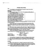
The velocity was calculated taking into account the distance travelled and the time taken for the cart to go down the wooden ramp. Mathematically:
With this formula, we use as an example the set of trials for height number 1 (0.084 m):
The same calculation was done for the other heights; results were recorded and put into a table:
With these results we can analyze the angle of the slope vs the average velocity in graph to understand their relationship. Thus the graph will include sin θ vs the average velocity, as shown below:
To analyze even further, the acceleration of the cart was calculated. For this calculation the following formula was used:
For example we use the velocity previously calculated, mathematically:
It is to be noted that the change in velocity was the same value as the velocity value obtained before, due to the fact that the cart started from rest. Therefore initial velocity was equal to 0.The same formula was used for the other set of results. This way the previous velocity table was expanded thanks to the inclusion of the acceleration values, as shown below:
With the use of this data, a final graph could be made representing acceleration vs the angle of the slope (sin θ is used again for more precision).
Conclusion
From the above graphs and a high R-squared value for the line of best fit it appears that within the uncertainties of the experiment, the acceleration of the cart as it goes downhill the wooden ramp is linearly related to the angle of the slope of the ramp.
From the hypothesis it was deduced that the relationship between the angle of the slope and the acceleration of the cart would be
Where a = acceleration, g = acceleration due to gravity (≈9.81 m s-2) and
the angle of the slope. The gradient of this linear relationship would then replace g in the equation.
If we take the any value of sin θ from the graph, in this case 0.219, we can calculate the value of the acceleration at that angle:
This value obtained should be the one shown in the graph, i.e. 0.970. The uncertainty for the acceleration is calculated using the maximum and minimum gradient, mathematically:
Maximum gradient = 7.65, therefore
Minimum gradient = 4.88, therefore
This way,
The value obtained from the experiment for the acceleration was 0.970, not the same value as the one that should be obtained from the calculations above. However, using the uncertainty for the value of acceleration 1.41 m s-2 this value can reach approximately 1.11 m s-2. This result is closer to the value obtained in the graph. It also is to be noted that the point 0.219, 0.970 in the graph is below the linear trend line which means that the value of 1.11 m s-2 isn’t an incorrect value, leaving room for a possible systematic error.
The results seem reasonable taken into account that the values measured were all relatively small, which can give a wider set of results. In addition, the R-squared value is high, maybe not as high as it should be but it still indicates a certain high level of correlation of the data to the linear graph. The analysis of the data gave proof to the hypothesis where the acceleration of the cart is directly proportional to the angle of the slope of the inclined plane:
, where if the value of sin θ increases (angle increases) the value for acceleration will increase too.
Evaluation
Measuring the lengths and heights for this experiment had small uncertainties; this was helpful for the analysis of the data later. The uncertainties that had a significant effect on the investigation were the ones for times measured. When measuring the time taken for the cart to go downhill a systematic error could’ve occurred, this could be classified as a parallax error. The time was measured with a stopwatch which was stopped when the cart hit the brick; depending on where the person is standing the time may vary slightly (the time of reaction to stop the stopwatch is also a common human error). However, this slight change in the results can affect the data because the range of times were all between 0.6 seconds and 1 second approximately (reason why results had to be precise), therefore if a small error was made then the further calculations would be affected as it was seen in the process of data. This didn’t affect the conclusion because the systematic error was taken into account and it was expected that the value would not be exactly as predicted.
The value for error bars helped to comprehend that results may not have been as accurate as it should have been. However, a trend line still passed through points of all the error bars, which helped to deduce that the relationship between the angle and acceleration was linear. The error bars for the height in the first graph were quite small compared to the uncertainty of time. There were no error bars for the values of the angles, this is because they are deduced mathematically from other results; if there was an uncertainty, it would be for the height or length measured, not for the calculation of the angle.
The line of the graphs should theoretically pass through the origin (intersect Y at 0). The uncertainties made it not possible for the line to do so, as the values for c in the line equations were 0.197 and -0.384 respectively. This means that there was a systematic error, as explained before, and it affected the graphing of the results.
Controlling the controlled variables didn’t cause any trouble at all. The length was measured and then the only thing to do was make sure that the ramp wouldn’t move. The same concept applies for the height of the ramp. By keeping these two variables controlled, the angle of the slope could be deduced and also controlled.
The distance travelled was always controlled by marking a line on the starting point, this way the cart wouldn’t travel more than the distance measured. The initial velocity was always tried to keep at 0 m s-1, by just stopping the cart at the starting point and releasing it as soon as the stopwatch started. There is a small chance that the stopwatch might’ve started after the cart was released causing the initial velocity to be a non-zero value, but it was never a big issue.
Time management wasn’t a problem either, as the trials all consisted in approximately 1 second. The part of the method that took most time to do was changing distance travelled. However, the experiment was straight-forward and it could be repeated several times when trials didn’t work out well or results didn’t seem to make sense.
Improving the investigation
Measuring the heights, lengths and distances for this experiment seem to work fine, therefore they didn’t need much improvement. The main thing to improve for this experiment is the measurement of time.
The best way to eliminate the systematic error for time measuring would be to use better technology instead of just a stopwatch. This means that instead of a stopwatch, photo gates could’ve been used. Using photo gates would be better as it measures the exact point where the cart starts and finish and it can give you the value for velocity and acceleration immediately. However, the initial velocity should still be controlled carefully as the photo gate cannot control that.
Other than that, maybe a greater amount of trials could’ve been made or maybe the use of a third person with another stopwatch could help too. There are also some external factors that could’ve affected the results, for example the friction force of the ramp, maybe at times it could’ve affected the time the cart took to go downhill. This force, however, doesn’t have a major impact on the results, but for a future experiment it should be negligible in order to obtain more accurate results.
The final improvement would be to use a longer distance, using more than half a meter approximately for this experiment resulted in small results for the time. For a future experiment, using a longer distance (of at least twice as the once used for this experiment), would give a wider range of data and it would be helpful for further analysis and processing of data.