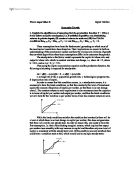
s ktα = (δ+n+g) kt
k* = (s/(n+g+δ))1/(1-α)
So, in steady state capital-labour ratio is related positively to the rate of saving and negatively to the rate of population growth. Predictions of Solow model are concerned about the impact of savings and population growth on real income. And it predicts not only the signs, but also the magnitude. We could say then that the savings rate and population growth affect growth only in the short run as well as the steady state level of y*. Convergence, therefore is conditional to the level of the savings rate and population growth and only productivity growth drives in GDP per capita in the long run. Policy, then, is unimportant for growth in the long run.
The amount of growth that can be explained by the model is given by the so-called Solow-residual:
A = Y - αK - (1-α)L
where all the terms on the right hand side are observable (possible to estimate directly)
Solow’s model analysed empirically
In his work titled “A Contribution to the empirics of economic Growth”, Mankiw, Romer and Weil investigate whether the data support the Solow model’s predictions concerning the determinants of the standards of living.
They assume g and δ constant across countries and s and n independent of country-specific factors shifting the production function and so they estimate the following function:
Ln (Y/L) = α - α/(1-α) ln(s) - α/(1-α) ln(n+g+δ) + ε
where ε is a country-specific shock
Their results imply that the Solow model is correct in some aspects like the signs of the coefficients on saving and population growth being as predicted by the Solow model; the ln(s) and ln(n+g++δ) coefficients being the same in magnitude but opposite in signs or the differences in saving and population growth accounting for a large fraction of the cross-country variation in income per capita, but not completely successful as the estimated impacts of saving and labour force growth are much larger than the model predicted.
The three main problems for the Solow model are:
-
The magnitude of international differences: assuming α = 1/3 implies that four times higher savings rate only implies twice as high level of production. But we need a model that is able to explain that income levels can vary by a factor of 10 at least. The differences in s and n to account for such differences are far too high. Because α/(1-α) must be higher, we need a higher α.
-
The rate of convergence for the Solow model gives us a 4 per cent, when the observed rate of convergence is roughly 2 per cent (α is again not large enough).
- The rates of return.
The augmented Solow model with human capital
They then proceed to enlarge the model including the human capital factor as a possible factor that would alter the analysis of cross-country differences.
The extended model therefore has the following shape:
Yt = Ktα Htβ(AtLt)(1-α-β)
where H is the stock of human capital and all other variables are defined as before
Solving for the steady state as we did before, we end up with the following results:
k* = [(sk(1-β) shβ) / n+g+δ ] 1/(1-α-β)
h* = [(skα sh(1-α)) / n+g+δ ] 1/(1-α-β)
Substituting these results into the production function and taking logs we have:
ln(Yt/Lt) = lnA(0) + gt - (α+β)/(1-α-β) ln(n+g+δ) + (α)/(1-α-β) ln(sk) + (β)/(1-α-β) ln(sh)
Which involves that income per capita depends on population growth and accumulation of physical and human capital.
They then estimate the model taking education as the main human capital form of investment. Although difficult to measure they conclude that adding human capital to the Solow model improves its performance and that it gives better estimates for the impacts of saving and labour force growth than the simple model.
Critics to the MRW work
The strong results in favor of the augmented Solow-model reported by MRW have been criticized by a number of newer studies. The criticism has been directed basically at shortcomings of the econometric methodology, the crude and inappropriate measure of human capital and that the fact that their model has a too static and narrow view of human capital. They mostly disagree with them taking the investment rates of physical and human capital as endogenous to the level of income as well as uncorrelated with efficiency.
Some of these disagreements are gathered in Temple’s paper titled “The New Growth Evidence” (1999). L. Pritchett also discusses the importance of education in MRW in his paper titled “Where has all the education gone?”.
Measuring human capital directly is extremely difficult so we need to settle for more or less appropriate proxies. Mankiw, Romer and Weil’s equation is formulation in such a way that we can use a measure of changes in human capital, rather than its level, as the right-hand side variable.
Mankiw, Romer and Weil’s choice of the secondary enrolment rate as their proxy is highly questionable. Why not include also primary education? Here, regional differences are much smaller. It is the difference in the educational attainment of the cohorts entering and leaving the work force that is relevant. Empirically, enrolment rates vary a lot over time. Klenow and Rodriguez prove that taking into consideration the primary school levels of the countries reduces the amount of differences explained by capital investment and give the technology differences the central role to explain cross-country differences.
Instead, many have suggested using estimates of human capital derived from micro-evidence on the returns to schooling.
In his work, Pritchett estimates a growth-growth equation (opposed to a Mankiw, Romer and Weil’s level-level equation) and his results give a fairly robust conclusion that there is a negative effect of schooling on growth in GDP per worker.
The strength of the results in MRW is thus strongly reduced.
Another critic to the Mankiw, Romer and Weil’s model point out the fact that they take a constant growth rate for all countries of 2% a year since 1960’s. Do we have to suppose that the reason for countries having negative growth rates since then is that they parted from levels above their steady states? This seems unlikely, as there is a lot of empirical and theoretical work to suggest that the primary reason that countries grow at such different rates for decades at a time is transition dynamics: a country with output below the level of its balanced-growth path will grow rapidly, whereas a country above its balanced-growth path will grow slowly.
The “new growth” theory
For a long time the standard growth theory of Solow dominated the thinking of the economists. The basic idea behind the neoclassical idea is simple: output depends upon two basic inputs: capital and labour. If we employ more units of labour to the fixed amount of capital, we will be subject to diminishing rates of return to labour. Of course, economist knew that this model is a simplification of reality. However this theory was accepted as an abstraction or a simplification of reality.
But as we have seen, many economists have been talking about issues of technology, for example, which was not clear in the initial model. Since there are only two inputs in the neoclassical theory, how can one explain changes in output that cannot be explained by the changes in the two inputs? The neoclassical answer was simple changes in technology explain any changes that cannot be accounted for by changes in these two inputs. But the problem was that a very large portion of the changes in output could not be explained by the changes in labour and capital.
New growth theory comes in many different variants. Some authors examine the accumulation of knowledge as another determinant of economic growth. Other authors would include human capital as well as physical capital in the initial model. The production function in the new growth theory can be expressed as
Y = F( K, L, H, A)
where H is human capital now
The new growth theory allows for the possibility of increasing returns to scale, whereby if all inputs are doubled, it is possible for output to more that double.
But the evidence suggests that much of the variation in income across countries comes from differences in output for given amounts of physical and human capital.
R. Hall and I. Jones (1996) examine economic levels instead of economic growth to find out the reasons of the differences in average growth rates across countries. Hall and Jones argue with some research-based theories of economic growth of P. Romer and others that say that the world economy grows because of technological progress through the invention of new ideas. But evidence proves that growth in all countries is driven by the underlying growth rate of world knowledge. The rapid growth of countries such as South Korea or Singapore would be explained more easily if we assume a rapid technologic knowledge transfer across countries.
If capital and technology can easily move across borders, there must be other factors that explain the differences in economic growth across countries.
A leading candidate hypothesis is that differences in these determinants of income are due to what Hall and Jones call social infrastructure. By social infrastructures, they mean institutions and policies that encourage investment and production over consumption and diversion.
“The infrastructure of an economy is the collection of laws, institutions, and government policies that make up the economic environment. A successful infrastructure encourages production. A perverse infrastructure discourages production in ways that are detrimental to economic performance.”
To measure infrastructure they use different variables: an index of the extent to which government policies favor production instead of diversion, a measure of the openness of the country of international trade, a measure of the extent to which the economy is organized around the principle of private ownership of the means of production, a measure of the fraction of the population in a country that speaks an international language and a physical measure of infrastructure, the distance of the country from the equator.
Their estimated model suggests that all the above variables are significant except for the type of economic organization (capitalist vs. statist).
Several pieces of evidence suggest that social infrastructure is important to differences in income among countries. East-West post war Germanys, North and South Korea are some examples of how similar countries (similar climate, natural resources, culture, etc) have experimented such different growth rates. Their social infrastructures however were very different. The market oriented economies were dramatically more successful economically that the communist ones.
The critics to the work of Hall and Jones agree that social infrastructure has a strong and significant effect on Y/L but argue about the difficulty of measure the social infrastructure. Measurement error is regarded as more problematic than taking social infrastructure as endogenous (using the mentioned variables like the distance from the equator of the percentage of population speaking a European language).
Conclusions
From the Solow model we derived that in steady state, output per worker is determined by the rate of investment in private inputs such as capital and skills, by the growth rate of the labour force and by the productivity of these inputs. Studies made with real data support the Solow hypothesis: rich countries invest a large fraction of GDP and time accumulating skills and capital. But we have seen that there are other factors such as the social infrastructures that encourage production and investment. If the social infrastructure of a country encourages diversion instead of production, the consequences can be detrimental. When entrepreneurs cannot be assured of earning a return on their investments, they will not invest.
How do we understand the rapid economic transformation of economies such as Hong Kong’s and Japan’s since the Second World War? Real incomes have grown at roughly 5 percent per year in these economies, compared to a growth rate of about 1.4 percent per year in the United States.
If differences in social infrastructure are a key determinant of differences in income across countries, then changes in social infrastructure within an economy can lead to changes in income. Fundamental reforms that shift the incentives in an economy away from diversion and toward productive activities can stimulate investment, the accumulation of skills, the transfer of technologies, and the efficient use of these investments.
REFERENCES
Barro, Robert J; Mankiw, N. Gregory and Sala-I-Martin, Xavier. “Capital Mobility in Neoclassical Models of Growth”, The American Economic Review, March, 1995.
Hall, Robert E and Jones, Charles I. “Why do some countries produce so much more output per worker than others?” Quarterly Journal of Economics, February 1999
Mankiw, N. Gregory; Romer, David and Weil, David. “A contribution to the Empirics of Economic Growth.” Quarterly Journal of Economics, May 1992, 107(2), pp. 407-38
Pritchett, Lant H. and Summers, Lawrence H. The Structural-Adjustment Debate. The American Economic Review, May 1993.
Romer, David. Advance Macroeconomics. McGraw-Hill 2001.
Romer, Paul M. “Endogenous Technological Change”. The Journal of Political Economy. October, 1990.
Romer, Paul M. “The Origins of Endogenous Growth”, The Journal of Economic Perspectives, Winter, 1994.
Solow, Robert M. “A Contribution to the Theory of Economic Growth”, Quarterly journal of Economics, 1956