Marginal Costs are fixed at P=53
The Graph below (fig 1) represents if Firm A were a monopoly using the above demand function. In order to maximize its profits, the firm would set its output where MR=MC. The monopoly output therefore is where Q=30. This correlates to a monopoly price of £83. Firm A’s Profit therefore is (30,000 *83) - (30,000 * 53) = £900,000
Cournot Model
Under the Cournot model, neither firm has complete knowledge of the behavior of the other. Both firms set output for a given period at the same time and only after revealing its output decision will a firm find out the output the other firm has chosen.
Cournot assumes the firms maximise their own profit subject to the constraint that the other firms output is fixed at its current level, or equivalently, both firms select their outputs so as to maximise profit subject to a zero conjectural variation. (i.e dQa/ dQb = 0). This means that if firm B sells Qb units of its good, firm A will supply Q- Qb (the whole market demand minus what is supplied by firm b). In effect, firm A is a monopolist over the remaining demand not satisfied by Qb.
To use our numerical example, if firm A believes that firm B will sell Qb=20, the demand curve for firm A will shift to the left by 20 (from D to D’). D’ is what is known as the residual demand curve.
If the price is £73 per unit, the total demand is Q=40. As firm B is supplying 20 units, firm A will supply Qa= Q– Qb = 40 – 20 = 20. At this point the pair are in Cournot equilibrium. Each firm is maximising its profits and neither wants to change its output.
To maximise its profit, firm A sets its output so that its Marginal revenue line relevant to its residual demand curve (MR’) equals marginal cost. By shifting its new demand curve appropriately, firm A can calculate its best response to any Qb. The graph below plots firm A’s best response curve, which shows how great a quantity firm A supplies for each possible Qb. Firm A will shut down and provide nothing (Qa=0) if it believes that firm B will provide Qb = 60.
If either firm is not on its best response curve, it changes its output to increase profit. Under the assumption of Zero conjectural variation, as time passes, duopolists tend towards a market equilibrium level that lies somewhere between the polar cases of monopoly and perfect competition. This is because each firm bases their supply decision upon the last known output by their competitor. As an example consider a new entrant into a market. Initially, the new entrant will keep output low in response to the original large output by the resident firm. However as time passes, the increased supply due to the entrant drives down prices and the initial monopoly producing firm cuts back production. As a result of this, the entrant will increase production. This continues until the two firms are in Cournot equilibrium.
For example, if firm A were to produce 30 and firm b produce nothing, it is not cournot equilibrium. Firm A is happy producing the monopoly output, but firm B is not on its best response curve. As the graph above shows, if firm B knows that firm A will sell Qa = 30, firm B will sell Qb=15. In response to this, firm A will cut back production and then firm B will increase theirs. This procedure will continue in they are both at equilibrium. Only at Qa= Qb=20 does neither firm want to change its behaviour.
This idea however does rely on the idea of discrete periods. There is substantial evidence to suggest that this is unrealistic and firms adjust output inter-period, generally increasing such that industry output is in excess of the expected Cournot equilibrium (Romano and Yildrim).
The Cournot equilibrium can also be solved algebraically.
As we know, P = 113 – Qa – Qb
The Residual demand line D’ is linear with slope -1, and as marginal revenue curves are twice as steep as their corresponding demand curve, the gradient of MR’ is therefore -2.
The Marginal Revenue function is thus
MR’ = 113 – 2Qa – Qb
Firm A’s best response (its profit maximising output), given Qb is the output that equates MR’ and MC.
MR’=MC
113 – 2Qa – Qb = 53
60 = 2Qa + Qb
30 = Qa + ½ Qb
Qa = 30 – ½ Qb eqn 1- Firm A’s best response curve
By the same reasoning, firm B’s best response function is
Qb = 30 – ½ Qa eqn 2
Subbing eqn 2 into eqn 1 gives:
Qa= 30 - ½ (30 – ½ Qa)
Qa = 30 – 15 + ½ Qa
¾ Qa = 15
Qa = 20.
Substituting Qa = 20 into eqn 2 gives Qb = 20, and this is Cournot equilibrium.
Total output, Q = Qa + Qb = 40.
Setting Q= 40 in the market demand equation (P= 113- Q) we confirm that the Cournot equilibrium price is £73
Therefore, Total Profit is (40,000*73) – (40,000*53) = £800,000. When in Cournot equilibrium this would mean a profit of £400,000 for each firm.
Stackelberg Model
The Stackelberg equilibrium is a scenario whereby there are two or more firms within the market but one plays the role of leader, setting quantity levels, while other firms are followers, reacting to decisions made by the leader. The leader has full knowledge of how its production decisions will influence the decisions of follower firms, whilst the followers are merely reactionary.
The follower in the Stackelberg model is always going to attempt to be a profit maximiser, given the constraints laid upon it by the dominant firm in the industry. Therefore, all its production decisions will be a function of the output produced by the industry leader. Thus, the leader predicts what the follower will do before the follower acts, and this allows the dominant firm to manipulate the follower and benefit at their expense.
In the below graph, D’ represents firm A’s residual demand curve (i.e Total Demand D minus the output firm B will produce as summarized by firm B’s best response curve). For example, if firm A sets Qa= 0, firm B’s best response would be Qb=30, it can be seen that at Qa= 0 , the residual demand curve intercepts the y axis at p= 83 which is 30 units to the left of demand, D, at that price.
Firm A will choose its profit maximizing output at Qa = 30, where MR’ (the marginal revenue curve that corresponds to the residual demand curve) equals marginal cost, £53. At Qa=30, the price is £68. Total demand at £68 is Q=45. Therefore, firm B produces Q- Qa = 45 – 30 = 15.
Thus in Stackleberg equilibrium, the leader provides twice as much as the follower and the combined profit is £675,000. The Stackelberg leader earns £450,000, and the follower £225,000.
Collusive Oligopoly
Collusion is a market condition whereby the firms trading opt to work as a team, collectively deciding the output between them. An example of such a cartel is OPEC. There is much debate over the benefits and likelihoods of firms colluding.
At Cournot equilibrium, both firms would produce 20 units each and each would receive a profit of £400,000. If our two example firms, Firm A and Firm B were to collude in order to maximise their profits they would produce where MR=MC. This is the same output as the monopoly output in Fig 1, and we can see this is where Q= 30. By cutting back production to 15 units each, they would increase profit to £450,000 each (i.e half of the monopoly profit of £900,000 for each firm). If the two firms collude, they could split the monopoly output in many ways. Firm A could serve all customers, i.e. Qa = 30 and Qb=0 and give firm B some of the profits, or they could split the monopoly output straight down the middle. All of these possibilities are shown on the above graph as the “contract curve”, where:
Qa + Qb = 96.
In a single period game, firms tend not to collude. This is because of a lack of trust. If the firms are going to engage in the game only once, each has an incentive to cheat on their agreement. If firm A believes firm B will produce Qb = 15, firm A can increase its profit from £450,000 to £500,000 by violating the agreement and producing Qa= 20.
In multiperiod games however, cartels do form. This is because unlike in a single period game, firms meet period after period and wayward firms can be punished.
There is therefore a clear incentive to form cartels in order to increase profits. To quote Adam Smith (Perloff, p432) “People of the same trade seldom meet together, even for merriment and diversion, but the conversation ends in a conspiracy against the public, or some contrivance to raise prices”. This would seem to suggest that collusion is inevitable.
However, cartels often fail because either the government forbids them or because each firm in a cartel has an incentive to cheat on the cartel agreement by producing extra output.
To sum up the three models, the total Stackelberg ouput , 45 , is greater than both Cournot, 40, and monopoly/ cartel, 30. As a result the Stackelberg price, £68, is lower than cournot, £73 and monopoly/cartel, £83. Thus, consumers prefer the Stackelberg equilibrium to the Cournot equilibrium and the Cournot equilibrium to a monopoly/ cartel here, and in any market where firms have identical cost functions.
The combined Stackelberg profit, £675,000, is less than the combined Cournot, £800,000, and monopoly/ cartel, £900,000, profits. The Stackelberg leader though, earns £450,000, which is more than it could earn through Cournot, £400,000. Total Stackelberg profit is less than total Cournot profit because of the Stackelberg follower earning less at £225,000.
Although firms would earn more through a cartel, it is difficult to suggest that collusion is inevitable, given the strong financial motivation to cheat on an agreement. However, the large numbers of laws that restrict collusion would surely not exist if it was not for the strong likelihood of it happening.
Bibliography
Nicholson, W,.2005. Microeconomic Theory, basic principles and extensions.9th ed. South Western.
Perloff, Jeffrey M., 2004. Microeconomics. 3rd ed. Pearson Addison Wesley
Frank, R,. 2000. Microeconomics and behavior. 4th ed. McGraw- Hill.
Hirshleifer, J,. Price theory and applications. 7th edition [online] available at:
URL:http://books.google.com/books?id=rYXyggvvs0wC&pg=PA279&dq=oligopoly&lr=&as_brr=3&ei=KQ6zR_8anLzMBKLt7boN&sig=uLY4ktm6DciEkLxfa_hRTE9TzPY#PPA290,M1
[accessed 11/02/08]
Romano and Yildirim (2002), on the endogenaity of Cournot- Nash and Stackelberg equilibria: games of accumulation [online] available at:
[accessed 14/02/08]