Tc = TINV(1-c;n-1) = Tc
Tc= 2.0076
Then, the confidence interval of 95% is equals to:
29.5962 – 2.0076 <= µ < = 29.5962 + 2.0076
27.5885 <= µ < = 31.6037
95% of the men get married for the first time between 27.5885 years old and 31.6037 years old.
h) Given that the sample size is greater than 50, now assume that you can estimate the population standard deviation, , with the sample standard deviation, s. Once again, compute a 95% confidence interval for the population mean, , of the age at which men are getting married for the first time using this estimation for .
E= Zc*(s/ Ѵ(n))
s = sample standard deviation for the sample
We have Zc = 1.96 for confidence = 95%, s = 7.0301 and n=52.
- E = 1.96 * (7.0301 / Ѵ52)
- E= 1.9108
Then, we have:
29.5952 – 1.9108 <= µ <= 29.5952 + 1.9108
27.6853 <= µ <= 31.507
Then, 95% of the sample is getting married for the first time between 27.6853 years old and 31.507.
3. After doing all of the above work, you discover some old research documents in your office from an intern 10 years ago that show an original belief that the population mean for the age men are getting married for the first time in your region is = 25. You are glad you have done the research anyway because you believe this has been changing over time. You decide to use hypothesis testing to determine whether your suspicions are correct. In advance, you have decided to use = 1%
a) State the null hypothesis H0 and the alternate hypothesis H1 for the mean .
Null hypothesis:
H0 : µ=25
H1 : µ > k (because according to the above work, we have µ= 29.5962)
b) Will you be using a one-tailed or two-tailed hypothesis test? If one-tailed, please state the direction.
I chose > because we have found µ= 29.6346
It is a one-tailed hypothesis test and it is a right-one tailed.
c) What is the test statistic, t, for this test?
t = (sample mean - µ) / (s/Ѵ (n))
t= (29.5962 – 25) / (7.0301 / Ѵ52)
t= 4.7145
d) What is the P-value for this test and how does it compare with ? Based on this result, what do you now believe about the population mean ?
H1: µ > k
P-Value = TDIST (|t|, n-1, 1)
In French = LOI.STUDENT (4.7145; 51; 1) = 9, 5658 E-06
So, we can say that P-value is under 1 percent, and then the hypothesis H is true.
Thanks to this result, we can say that, in average, the population gets married for the first time after 25 years old.
e) Given the large sample size, you can also compute the P-value with the normal approximation. If you estimate with s, what is the P-value using this method? Comparing the P-values, is the approximation a good one?
If we estimate σ with s, we have σ equals to 7.0301.
Then, P-Value = 1- NORMDIST (mean, k, σ/ Ѵ(n), TRUE)
P-Value = 1 - =LOI.NORMALE (29.5962;25;7.0301/7.2111; VRAI)
P-Value = 1- 0,999998789
Then, we have P-Value 1 = 9, 5658 E-06 and P-Value 2 = 1, 21148E-06
So P-Value 1 is close to the P-Value 2, then we can conclude that the approximation in this case is a good method.
f) What if your original level of significance was 5% instead of 1%, is there enough evidence to reject the null hypothesis?
P-Value 1 = 9, 5658 E-06
We cannot reject the null hypothesis because we don’t have enough evidence.
4. You decide to try another way of testing whether the population mean, for the age at first time of marriage has been changing over time. You decide to look at the data you have available and see if you can run an ANOVA test. You decide to obtain a random sample of marriage licenses from ten years earlier in 2001 as follows:
17 17 18 19 19 19 20 20 21 21 22 22 22
23 24 25 25 26 26 26 26 27 27 27 27 27
28 28 28 28 29 29 29 30 30 30 30 30 30
31 31 31 32 32 32 33 33 35 37 38 40 41
Run an ANOVA test and include the output. What can you conclude?
We can note that, thanks to this ANOVA test, the mean between 2001 and 2011 has increased of more than 2 years. The men get married then later than before. Indeed, the average age was of 27.26 years old in 2001 whereas it is of 29.59 in 2011.
5. Dolomites Pizza Company has found that its pizza delivery time is distributed approximately normal with a mean of minutes and a standard deviation of = 3 minutes. Their motto is “Pizza within one hour or it’s free!”
Y = 20 minutes
W = 675 pizzas
a) You’ve just ordered a pizza from Dolomites. What is the probability that it will be on time (hint: arrive in one hour or less)?
P(X<= 60) = NORMDIST(x, mean, standard deviation, TRUE)
- = NORMDIST (60, 50, 3, TRUE) (in French =LOI.NORMALE(60;50;3;VRAI) )
= 0.9995
Then, the probability for that the pizza will arrive on time is of 99.95%
b) What is the probability that it will arrive in less than Y minutes? SEE THE DATA APPENDIX FOR YOUR VALUE OF Y
Y = 20 minutes
P(X<= 20) = NORMDIST(x, mean, standard deviation, TRUE)
- = NORMDIST (20, 50, 3, TRUE) (in French =LOI.NORMALE(20;50;3;VRAI) )
= 7, 61985E-24
That is to say it is quasi impossible that the pizza arrive in less than 20 minutes.
c) What is the probability that you will receive a free pizza?
The pizza has to arrive after 60 minutes to receive a free pizza.
P(X>= 60) = 1 – 99.95%
P(X>= 60) = 0.05%
Then, the probability to receive a free pizza is of 0.05%
d) In a typical week, Dolomites delivers W pizzas. How many will likely be free? SEE THE DATA APPENDIX FOR YOUR VALUE OF W
W = 675 pizzas
Then, on 675 pizzas, 0.05% will be free (according to the probability).
0.3375 pizzas will be free, that is to say quasi no one.
e) In a cost-cutting move, the company has reduced the number of drivers available to deliver pizzas, which has led to longer and less predictable delivery times. As a result, the delivery times are now distributed with a mean of 55 minutes and a standard deviation of 5 minutes. You must decide if the motto needs to change. Specifically, if the company wants to give free pizzas no more than 10% of the time, what should be the guaranteed delivery time? What would you recommend?
We have a mean of 55 minutes and σ=5minutes, then:
P(X<=60) = NORMDIST (60, 55, 5, TRUE)
P(X<=60) = 0.8413
P(X<=60) = 84.13%
- In this case, the probability that the pizza will arrive with less than one hour is of 84.13%
.
Then, the probability that the pizza is free is of 15.87% (100% - 84.13%)
15,87% > 10%, then we have to change the motto.
We have to ask us what would be the necessary delivery guarantee time to ensure that only 10% of the pizza could be free. For that, we have to use the NORMINV function:
P(X) <=90% = NORMINV (probability, mean, standard deviation)
= LOI.NORMALE.INVERSE (in French)
P(X) <=90% = 61.4077
Then, I will recommend to the pizzeria to guarantee a time of 62 minutes for the delivery. In this fact, the probability that the customer will have a free pizza will be of less than 10%.
6. Zony is a well-known electronics company specializing in all kinds of audio equipment, such as DVD players. Based on extensive testing and data collection, it is determined that the average life of the Zony portable DVD player is approximately normally distributed with a mean = 28 months and a standard deviation = 5 months.
You are sitting in a meeting with the CEO who says she doesn’t care about these numbers and , she wants to get a practical description of how long these DVD players are lasting. You do not have access to Excel but you remember the rule of thumb/empirical rule and think you can add something valuable to the conversation. You decide to compute the following:
- Between what two values of X, will approximately 68% of the values be? In other words, 68% of the portable DVD players sold will last between how many months?
Thanks to the rule of thumb, we know that we have 68% of the sample which is between µ - σ and µ + σ.
Then, in this case 68% of the last Zony portable DVD players have been sold between (28-5 = 23) 23 and (28+5 = 33) 33 months.
- Between what two values of X, will approximately 95% of the values be?
If the value is of 95%, then X will be between:
µ - 2σ <= X >= µ + 2σ
28-10 <= X >= 28+10
18 <= X >= 38
Thus, according to the rules of thumb, 95% of the DVD Player of Zony will last between 18 and 38 months.
- Between what two values of X, will approximately 99.8% of the values be?
If the value is of 99.8%, then X will be between:
µ - 3σ <= X >= µ + 3σ
28-15 <= X >= 28+15
13 <= X >= 43
Thus, according to the rules of thumb, 99.8% of the DVD Player of Zony will last between 13 and 43 months.
- Do you expect a DVD player to last more than 2 years? Explain.
2 years = 24 months yes I expect a DVD player will last more than 2 years because the average life time of the DVD players is of 28 months.
- Do you expect a DVD player to last less than a year? Explain.
We have seen that 99.8% of the DVD last between 13 and 43 months. Then, the probability for that the DVD last less than 13 months is of 0.02% (1-0.998).
Then, as the probability is very low, we can say that I do not expect that a DVD player last less than 1 year.
f) Based on your answers above, what do you say to the CEO?
Their DVD players have a good long life time.
g) The CEO thanks you for your comments saying, “Finally, someone who can take the research numbers and tell me practically what it means.” She adds, “Zony guarantees a full refund on any defective DVD player for 2 years after purchase. What percentage of our total production will we expect to replace?
X<= 24
P(X<= 24) = NORMDIST (24; 28; 5; TRUE)
P(X<= 24) = 0.2118
P(X<= 24) = 21.18%
According to the probability, the ^percentage of our total production we will expect to replace will be of 21.18%.
h) If we sold 40,000 DVD players this year, how many might come back to us with problems?
You excuse yourself to get to your laptop and assure the CEO, you will be right back with an answer.
Then, 8472 DVD players might come back to the factory.
i) Do you have anything in particular to recommend to the CEO?
The 2 years of guarantee are too much. Indeed, if the company guarantees their DVD 2 years, lots of DVD will come back in the factory with problems. That is why, it will be good for the company to reduce the last of the guarantee a 18 months or 1 year.
7. Marco’s Auto Insurance Company took a random sample of 470 insurance claims paid out during a 1-year period. The mean claim paid for that sample was x-bar. Assume = $250 for the distribution of insurance claims. SEE THE DATA APPENDIX FOR YOUR VALUE OF x-bar.
a) Find a 90% confidence interval for the mean payment.
Thanks to excel, we have to use the confidence formula:
Confidence (1-0.9; 250; 470) = E
Then, E= 18.9679
Then, 90% of the mean payment are between (1325 – 18.9679) 1306.0321 and 1343.9679 (1325 + 18.9679).
b) Find a 95% confidence interval for the mean payment.
Thanks to excel, we have to use the confidence formula:
Confidence (1-0.95; 250; 470) = E
Then, E= 22.6016
Then, 95% of the mean payment are between (1325 – 22.6016) 1302.3984 and 1347.6016 (1325 + 22.6016).
c) For the above problem, find the sample size, n, necessary for a 99% confidence level with maximal margin of error, E = $20.
The confidence formula is: E= Zc*(s/Ѵ (n))
Thanks to the data, we have:
20 = 2.58*(250/ Ѵ (n))
20/2.58= 250/ Ѵ (n)
7.7519/250= Ѵ (n)
Ѵ (n) = 0.0310
N = 0.1760
8. A pasta making machine is set to cut pasta noodles at a thickness of =0.05 inches and standard deviation = 0.003 inches. This kind of precision is difficult to maintain because high production quantities each day may affect the alignment of the machine. In order to avoid this problem, the machine is tested every day with a sample of n=10 pieces of pasta. Today’s sample had a sample mean X = 0.053 inches. At = 5% level of significance, is the machine out of alignment?
a) State the null hypothesis and the alternate.
Null hypothesis ➔ H0= 0.05 (with k = 0.05)
Alternate hypothesis: H1➔ µ does not equal k
b) Is this a one-tailed or two-tailed test?
This is a two-tailed test.
c) What is the P-value?
σ is known, then:
- P-value = 2*NORMDIST (mean, k , σ / Ѵ(n), TRUE)
if x<k
Then,
P-Value = 2*LOI.NORMALE (0.053; 0.05; (0.003/B6); VRAI)
P-Value = 2*0.9992
P-Value = 1.9984
And:
- P-value = 2*(1-NORMDIST ((mean, k , σ / Ѵ (n), TRUE))
if x>k
Then,
P-Value = 2*(1- LOI.NORMALE (0.053; 0.05; (0.003/B6); VRAI))
P-Value = 2*(1-0.9992)
P-Value = 2* 0.0008
P-Value = 0.0016
d) How does the P-value interval compare to ?
P-Value > α ➔ I don' reject the Hypothesis 0 and the hypothesis x < k is impossible.
e) Does the evidence support the hypothesis that the pasta machine is out of alignment?
f) Does your answer change at the 2% level of significance?
No, my answer will not be changed because 1.9984 > 0.02 and 0.0016 < 0.02, then we don’t have enough significance to reject the hypothesis.
9. Suppose you suspected that there is a relationship between the total number of jobs available in a city and the number of entry-level jobs in the same city. You are provided with a sample of data points for six cities in France. SEE THE TABLE IN THE DATA APPENDIX FOR YOUR DATA SET
Number of total jobs 16 33 49 28 49 25
Number of entry level jobs 2 3 6 5 9 3
a) Decide which variable you wish to be the dependent variable and which the explanatory variable. Why did you make this selection?
We want to know if there are a relationship between the number of entry level jobs in a city and the number total jobs. Then, we will take as explanatory variable the number of total job and as the dependant variable, the number of entry level jobs. We are going to see if there is a correlation between the number of total job and the number of entry level jobs.
b) As in the examples in class, create a scatter plot of the data. Be sure to include the value for R2 and the trendline.
Y = 0.166x – 0.8681
R²= 0.7356
c) Based on the value for R2, what do you conclude?
R² represents how well the linear regression fits to the data.
In our example, we have R²= 0.7356 which means the linear regression fits to our sample of data with a degree of 73.56%. We can be confident with our estimations.
d) Run a regression using ToolPak in Excel (or its equivalent). Please include the output values. What do you conclude from the output?
We can conclude that the two variables are linked.
e) Can you think of another explanatory variable to include which might improve the value for Adjusted R2?
We can also add another explanatory variable such as the rate of unemployment or the average wages of the population in the city.
f) If a particular city has a total of 42 jobs, how many would you predict to be entry-level?
We have y = 0.166x – 0.8681
So we have y= 6.10
I would predict 6.1.
10. During our seminar, we covered a wide-variety of topics in business statistics. Think about the different tools we learned about and comment which ones you believe will be most useful in your area of interest (marketing, finance, etc.) and why. Any specific example which you can provide would enhance your answer.
The last year, I specialized myself in the finance area. The wide varieties of topics we have treated during seminars have been very interesting to me. Finance and statistic are linked, because they are complementary to each other. Investment requires statistical studies which are provided by the use of business statistic analysis. These studies are very useful; indeed they provide confidence for investors and portfolio managers. Linear regression combined with financial ratios such as expected earnings, market positions, dividends growth rate, can tell us how the share price might move in the future. If our linear regression based on our estimated sample of data is closed to the reality (R² ratio), portfolio managers can easily convince investors to invest in their funds. The degree of confidence given by our statistical analysis tells us how much and/or in which asset the manager should invest in. Business statistical analysis should be use with fundamental analysis in order to achieve the best forecasts of the future company’s growth. I found these seminars very interesting, my knowledge in this area are now improved and I can use different tools on Excel that I did not know before your seminar.