Compare and contrast the Capital Asset Pricing Model and the Arbitrage Pricing Model.

University Degree Business and Administrative studies

Introduction

This essay is aim to compare and contrast the CAPM and APM . Both of these two model are equilibrium asset pricing model .To understand the similarities and differences between them , Firstly, we will derive and interpret CAPM and APM . Then compare them in different sides and rise the limitation of the CAPM . Finally , we will analysis whether and how the APM can avoid these problem .

Derive CAPM and APM

CAPM:

The Capital Asset Pricing Model is an equilibrium model of asset pricing, it states that the expected return on a security is a positive linear function of the security’s sensitivity to changes in the market portfolio’s return.

To derive the CAPM, first we must assume away the complexities since the real world is sufficiently complex, and focus on the most important element .

These assumption are as follows:

Investor evaluate portfolio by looking at the expected returns and standard deviations of the portfolios over a one-period horizon.
Investors are never satiated, so when given a choice between two portfolio with identical expected standard deviation, they will choose the one with the higher expected return.
Investor are risk-averse, so when given a choice between two portfolio with identical expected return. they will choose the one with the lower standard deviation
Individual assets are infinitely divisible , meaning that an investor can buy a fraction of a share if he or she so desire .
Investor may either lend or borrow money at the same risk free rate .
No taxes or transaction costs.
Investor have same one-period horizon.
Information can be transmit to all investor freely and instantly .
Investors have same expected returns, standard deviation, and covariance of securities

The CAPM becomes an extreme case by made these assumptions. All investors have same information and prospectors for the securities. There are no friction to impede investing, security market is an perfect market. This is imply that all investor, in equilibrium, would obtain the same tangency portfolio which is the optimal one, because investors have same expected return, standard deviation and covariance . Also, the linear efficient set is the same for all investors. Since all investor face the same efficient set, the only reason they will select different portfolio is the difference curves are different. Although the chosen portfolio is different ,nevertheless the chosen combination of risky securities have same relative proportions. This feature is known as separation theorem.

Another feature of CAPM is that in equilibrium each security must have a nonzero proportion in the composition of the tangency portfolio. In equilibrium, the proportions of tangency portfolio will correspond to the proportions of what is known as the market portfolio, defined as : A portfolio consisting of an investment in all securities. The proportion invested in each security equals to the percentage of the total market capitalization represented by security. ( sharp 230&920 )

E( R )

E( Rm ) M

Figure 1

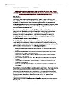
The market portfolio plays a important role in the CAPM because the efficient set consists of risk free borrowing/lending and the investment in the market portfolio. As can be seen from the Figure 1, the tangency portfolio M is denoted as the market portfolio, and R represents the risk free rate of return. Therefore, the efficient set consists of a single straight line , emanating from the risk free point R and passing through the market portfolio M. This line RM is called capital market line ( CML ). Since the slope of CML equal to the difference between ...

This is a preview of the whole essay

( 1 )

The CML shows the relationship between the expected rate of return and risk of return( measured by standard deviation ). Individual risky securities always plot below the CML since the single risky security when held by itself is an inefficient portfolio. However, CML does not give the expected return to inefficient asset. This can be solved by capital asset pricing model .

Since the market portfolio M is efficient , the expected return of any asset i satisfies:

( 2 )

where : ( 3 )

Therefore, the equilibrium relationship between risk and return can be written as :

( 4 )

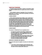
E( R ) E(R)

E(Rm) M E(Rm) M

R R

Figure 2.a Figure 2.b

We gave a graphic treatment to CAPM formula (4) , the figure 2 shows a linear relationship which termed the security market line ( SML ). Both figure 2.a and 2.b show the linear variation of E( R ). Figure 2.a expresses it in covariance form ,M corresponds to the point ; 2.b shows it in beta form and M corresponds to the point =1. Therefore, efficient set plot on the both CML and SML , but inefficient set plot on the SML below the CML.

APM:

The arbitrage pricing model is an equilibrium model of asset pricing . It states that the expected return on a security is a linear function of the security’s sensitivity to various common factors. This model does not require the assumption that investor evaluate the portfolio on the basis of means-variance.

Assumption:

Investors will seize the opportunity, which can increase the return of their portfolio without increase the risk.
Security returns are related to an unknown number of factors.
Homogeneous expectations

The APM is basis on the factor model and require the returns on any asset be linearly related to a set of index:

(5)

Here, ai is the expected return when all indices have a value of zero; bik is the sensitivity of asset i’s return to the kth index;Rk is the value of the kth index that impacts the return on asset i . This is just like the Market Model except that there are K sources of influence. Each source of influence can be referred to as a risk factor.

We can find the APM equation by Equilibrium condition (market clearing).that is to say there are no opportunities for arbitrage. If any asset is either over-priced or under-priced there is an opportunity for arbitrage

( 6 )

and it can be written as :

( 7 )

To derive the APM , we assume k source risk, then the return generating equation is :

it is also the equation (5)

since the k source of risk are independent , any n-asset portfolio can be written as :

(8)

write (8) as a zero-mean version ,and take the expectation of (5), the equation as below :

(9)

we subtract (9) from (5) : ( 5 ) - ( 9 ) , and obtain

where is the mean-zero return to risk factor k. Then the portfolio return can be written as :

From the APT, the arbitrage portfolio increase the expected return of portfolio without increase its risk. First of all, it is a portfolio that does not require any additional funds from the investor. Second, an arbitrage portfolio has no sensitivity to any factor. Finally, it should also have zero nonfactor risk . These features, in mathematical can be written as :

uses no wealth (costless)

has no systematic risk.

has no non-systematic risk

Therefore, by apply the arbitrage portfolio features above and its weights to the mean-zero equation for the portfolio return , we can calculate : . That is to say, the arbitrage portfolio return is certain. Now, we can write the expected return to any asset as a linear combination of a constant term and its:

. (10)

This is also the equation of the Arbitrage Pricing Model.

This equation states that there is a linear relationship between the expected return and sensitivity of factor . When the asset i is riskless , mathematically, . The asset will earn the risk free rate of return, that is .

To interpret , we assume that portfolio only sensitivity to risk h and have zero sensitivity to all other factors. Then it is not a arbitrage portfolio but a index portfolio representing risk factor h . These situation imply :

and .

Then the property of this portfolio can be written as:

The general form of , in the same way, can be written as :

we substitute the and the into the APM equation (10):

Compare the CAPM and APM :

After derive the CAPM and APM, now we will compare this two model. By definition, both of these two model are equilibrium model of asset pricing, but what are the similarities and differences between these two model ? First of all, we will focus on the assumptions of them.

Assumptions:

The capital asset pricing model is based on a serial assumptions, including the assumptions of the mean-variance model and some other additional assumptions about the behaviors of investor and the existence of perfect security market. These assumptions indicate that all investor hold the same efficient portfolio of risky asset, that is the identical opportunities. However, these assumption also a restriction of CAPM since the critical assumption of mean-variance are violated, say the normally distributed return and the quadratic utility functions.

In contrast, the arbitrage pricing model requires less assumptions than CAPM, the primary assumption is that all investor will Investors will seize the opportunity, which can increase the return of their portfolio without increase the risk. The APM does not use the mean-variance model ,it base on the factor model . Then there is no assumption about distribution of returns and only assumes non-satiation, diminishing marginal utility and expected utility, but does not require quadratic utility.

Then in the assumption term, the APT is more consummate and convenient than the CAPM.

The Equilibrium Concept in The CAPM and APM:

Both of these two model are equilibrium model of asset pricing, but the CAPM is only defined at equilibrium. It does not explain how the market move to equilibrium. Equilibrium in the CAPM is defined by imposing market-clearing on the optimal portfolio choice of the mean-variance model. In the equilibrium, each security must have a non-zero proportion on the tangency portfolio T . It is the market portfolio. If all investor purchasing portfolio T and T does not include an investment in security S , then nobody investing in S. Therefore, the price of S will drop causing the expected return of S increase until the market portfolio T has a non-zero proportion of S . Finally, when the price adjustment stop, the market will be in equilibrium.

In contrast, the Equilibrium in APM can explain how the market moves to equilibrium ,it is achieved by the process of arbitrage imposed on an assumed multi-index returns-generating process, that is to say market moves to equilibrium when there are no opportunities for arbitrage. By definition, arbitrage is the process of earning riskless profits by taking advantage of different pricing of same stock. In another word, sale a asset at a higher price and buy it at a lower price simultaneously. If any asset is either over-priced or under-priced there would be an opportunity for arbitrage and can earning a costless, riskless profit. Since the homogeneous expectations that all investor would exploit this opportunities for arbitrage and the market will move to equilibrium.

The Risk Factor :

In the CAPM ,from the equation (4),

E(Rm) is the return to the market portfolio and it is also the only risk factor which defined as the systematic risk .However there are many other influence which can impact the return of the portfolio, and not all the portfolio are marketable. “The CAPM rests on an unobservable market portfolio that has a clear economics meaning .”

In the APM, from the equation (5),

the Rik also the return to portfolio. These portfolio represent K risk not only include systematic risk but also represent non-systematic risk. Then “the APM rests on observable indices that have unclear economics meaning.”

The Test Of CAPM and APM:

Many scholars did the testing work to the CAPM , but the Roll’s critique said that results of these test are not necessarily the case.

Suppose z and q are frontier portfolios and z has zero covariance with portfolio q. Then for any other portfolio or asset p, in mathematical:

this equation is not need to be tested. It is true for any observed efficient portfolio, m, and orthogonal portfolio z. Then the test is to test whether the market portfolio is an efficient portfolio by the equation:

Since the market portfolio is unobservable so this relationship is tested for a proxy to the market portfolio and the CAPM is not tested.

The APM is based on the factor model not reliance on the market portfolio. Most test of APT other than factor analysis is used to obtain the for testing APT. The result suggests that APT is a useful model for explaining relative expected return and the multi-index model does a better job than both single-index and CAPM.

Syntheses of CAPM and APM:

The existence of multifactor model is not necessarily in consistent with CAPM. In the simplest case, if the return generated by single index model and the factor is market portfolio, then CAPM will hold :

(a)

If returns are generated by single index model but the factor is not the market portfolio and CAPM also hold :

(b)

If returns generated by a multi-index model , it is also possible for the CAPM to be hold. Suppose a two factors model , the equation (b) can be written as:

then the APT equilibrium model for this multifactor model return generating with a riskless asset is :

( c )

The equation ( C ) shows that security expected return is related to beta and sensitivities. If the CAPM is the equilibrium and holds for all securities and the index can be represented by portfolio of securities then

substitute to equation (c ),

This equation imply that betas will related to sensitivities in the following linear relationship:

Then it results in the expected return of E(Rm) being priced by CAPM :

“In conclusion, the APT solution with multiple factors is fully consistent by the CAPM.”

Conclusion:

After derive and compare the CAPM and APM, we know that both of them are equilibrium model of asset pricing . The APT promises to supply us with a more complete description of return than the CAPM . Because of there are some problem and limitation with CAPM such as : 1. The restrictive assumptions, since the critical assumptions of mean-variance model are violate ; 2. The market portfolio playing a special role in the CAPM, it contains all asset and known to be the only risk factor of CAPM; 3.the test of CAPM, according to Roll’s critique it is a test for M ; 4. The CAPM defined at equilibrium , can not explain how the market moves to equilibrium .

The APM can avoid most of these problem and limitations. It use less assumptions and based on the factor mode but not identify the factors . APM also can explain how the market moves to equilibrium that is by the process of arbitrage. Therefore the APM is more general than the CAPM . However, they are not necessarily inconsistent with each other. If security’s returns are generated by a factor model and simultaneously hold the CAPM , the security’s beta will depend on the sensitivity to the factors and the beta value of the factor with the market portfolio.