D (pi) if pi<pj
Di (pi, pj) = ½ D (pi) if pi=pj
0 if pi>pj
(Tirole 210)
How each firm will react in this situation? As seen in above analysis each firm optimal price will depend on what it conjectures other firm will choose. So each firm treats price of the rival as given, and then aggressively sets price, just under rival’s price (pi-ε-MC), to steal market share from the rival. As it can be seen because duopolistics’ products are perfect substitutes whichever firm sets the lowest price it gets all the demand. Specifically, if firm i charges price pi which is lower than the price of firm j, pj, it gets whole market demand D (pi) whereas firm j’s demand is zero.
Diagram 1
Bertrand Model: Equilibrium (Lecture Notes)
The final outcome of this game - referred as Bertrand or Nash equilibrium - is a pair of prices pi, pj such that each firm’s price maximizes that firm’s profit given the other firm’s price. This unique solution to Bertrand’s game is known as The Bertrand paradox, which argues that a unique equilibrium exists within these strict assumptions, and it is characterized by the two firms charging the perfect competition price (i.e., the marginal cost), hence forcing economic profits to zero (pi=pj=MC). (Tirole, p.210) (Diagram 1) Once again this result holds only if we have identical firms with same MC, producing homogenous goods and having no capacity constraints. Moreover this result is valid and for only two competitors and in the case where we have n number of firms.
The Cournot Model
One of the first models of oligopoly markets was developed by French mathematician Cournot, whose book Bertrand was reviewing when he put forward the model of the last section, and it represents probably the most widely used model of non-cooperative oligopoly. In this model a firm's profit maximizing decision depends on the output of the other competitor and not on the prices as it is the case with Bertrand model. In Cournot model of duopoly prices are set by an auctioneer such that demand equals supply. In this chapter I will start the discussion with the duopoly case and then consider what happens as the number of firms increases.
Duopoly Case
Let us consider a two firms game where there is no entry and where firms produce identical (homogenous) products so that total industry output is Q=q1+q2, where firm 1 produces q1 and firm 2 produces q2. We also assume that market demand function is a linear function of price, Q=1000-1000p, and that both firms have constant marginal cost, MC, of 28 pence per unit and no fixed costs. Moreover firms are not capacity constraint. (Carlton at all, pp.157-9)
Which level of production will each firm choose, In Cournot model, this depends on its conjectures about other Firm’s behaviour. Each firm will thus try to maximize its profit given the quantity chosen by other firm. As example Firm 1 will face the residual demand curve q1=Q(p)-q2, which is market demand curve minus the expected output of Firm 2, q2. This can be seen on the following Diagram 2.
DIAGRAM 2
It can be seen that the residual demand curve is obtained by shifting the market demand curve by q2 (240) units to the left. Firm 1 now has a monopoly over those customers that have not been served by Firm 2 and so it chooses q2 where its marginal revenue based on derived residual demand curve intersects its marginal cost curve. Since this choice will surely be not equal to the outcome of perfect competition and so the Cournot outcome will not be socially efficient.
This relationship can be summarized by best-response function (qi= Ri (qj)) which shows best choice of the firm given its conjectures about the action its rival takes.
Solving our example we get that Firm 1’s best response function is q1= R1 (q2) =360- q2/2 and since those two firms are symmetrical Firm’s 2 best response function is q2=R2(q1)=360- q1/2 i.e. how much firm 2 will produce depends on what does it expects that Firm 1 will produce.(on diagram below)
Derivation
(1) B1 = p(Q)q1 - .28q1 = [1 - .001(q1 + q2)]q1 - .28q1
(2) B1 = q1 - .001(q1)2 - .001q2q1 - .28q1 = q1(.72 - .001q2) - .001(q1)2
(3) MB1 /Mq1 = (.72 - .001q2) - .002q1 = 0
(4) q1 = (.72 - .001q2)/(0.002) = 360 - .5q2 = R1(q2)
DIAGRAM 3
q1
720
q1=R1 (q2)
360
Cournot Equilibrium
240
q2=R2 (q1)
240 360 720 q2
As diagram 3 illustrates we have equilibrium where those two best-reaction functions cross once and so in our case in the equilibrium quantities produces by both firms are identical q1= q2=240. At this point firms choose quantities given what they conjecture the other firm is doing; and those expectations are correct. This point is known as Cournot equilibrium. More generally “A Cournot equilibrium is a list of output levels produced by each firm and the resulting market price so that no firm could increase its profit by changing its output level, given that other firms produced the Cournot output levels. Thus, Cournot Equilibrium output levels constitute Nash equilibrium in a game where firms choose output levels.” (Shy, p.99)
We can compare this result with monopoly and perfect competition. In fact Cournot equilibrium lies somewhere between the extremes of monopoly and perfect competition. This can be shown on simple diagram. (Diagram 4)
Diagram 4 (Cabral, p.112)
q1
qc
q1 + q2 = qc (perfect competition)
qm
N q1 + q2 = qm (monopoly)
qm qc q2
“As it can be seen duopoly output is greater than monopoly output and lower than perfect competition output. Likewise, duopoly price is lower than monopoly price and greater than price under perfect competition.” (Cabral, p.112) This statement is supported by our case. It can be calculated that the cartel output is 360 and the cartel price is 64 pence, while the Cournot output is 480 and the price is 52 pence (19% lower than cartel) than in the cartel equilibrium. Therefore firms are better off when they form a cartel than when they engage in Cournot competition; however consumers are better off at the Cournot equilibrium than if we have monopoly (cartel). Moreover under perfect competition we have output of 720 units and price of 28 pence which surely further supports our statement. (Carlton at all, p.165)
N-firms
As I mentioned before Cournot model will give different result if more than two firms engage in the game. Again we can use same analysis that we have used before. In this case first step would be to take one firm and calculate its output level as a function of the output levels of all other firms. So Firm’s 1 best-response is q1=R1(q2,q3,….qn). And so if all firms produce identical output than Firm’s 1 best-response can be rewritten as q1=360-q(n-1)/2. This will also hold for all other firms, since we assumed they are identical. So solution for Cournot equilibrium will be q=720/(n+1) and p= (1+0.28n)/(n-1).
Therefore by manipulating with number of firms we can see how industry output and price changes. The effect of additional firms on q and p is very strong but it becomes lees influential as number or competitors increases. In the case of Cournot duopoly we saw that the price is 86 percent above the competitive price. But if we take n=10 firms we can calculate that new price will be much closer (just 23% higher) to perfect competition (with 50 firms only 5% above pc). If we further increase number of firms p will be closer and closer to perfect competition price. (Carlton at all, p.165)That is, in Cournot equilibrium, as number of firms grows indefinitely, the output level of each firm approaches the competitive output level and so price approaches competitive price. This is natural to expect since with many other firms in competition individual firm has only small influence on the price and so acts almost as a price taker. Consequently, consumers are better off (lower price and greater consumer surplus) and firms are worse off (lower profits) as the number of firms increases i.e. as in the perfect competition case.
Bertrand versus Cournot
In previous two sections we have analyzed the same industry where in the Bertrand model firms use prices as actions and where in Cournot model firms use quantity produced as actions. In general, our analysis has shown that these two models give different prices and quantities at equilibrium. Whereas in Cournot duopoly model firms make positive profits having price above MC, in Bertrand model firms make zero profits as is the case in perfect competition model. However the outcome becomes more similar as more firms enter the market under Cournot market structure. If number of firms is large enough than Cournot market structure yields approximately the same price and output as competitive market structure. Therefore this analysis supports the statement from the title that Cournot and Bertrand competitors are behaving identically when the number of Cournot competitors increases.
However this holds only under strong assumptions of no capacity constraints, constant marginal costs, if the market last only for one period and if we have homogenous products. If some of these assumptions were relax then price competition among several firms would not reach competitive outcome and our justification will have different outcome. As example if firms had different MCs than only firm will lover MC would be producing in Bertrand’s model and it will set a price just above its competitor’s MC, which is higher than perfect competition price, and be only seller in the market. Similarly for all other cases prices will differ and they will not be equal to MC. (For other cases see Tirole pp.211-2, Cabral p.105)
Conclusion
According to Bertrand model price competition between symmetric firms yields competitive outcome and this results hold no matter how many firms engage in competition. On the other hand Cournot model showed that the price under duopoly is greater than that under perfect competition and lower than monopoly price. However contrary to Bertrand model, it exhibits negative relationship between number of firms and profitability. We have shown that in fact if number of firms is extremely large, in Cournot model of oligopoly, industry price and industry output approach socially optimal level as in the perfect competition. Therefore we have shown that under certain assumptions and with large number of firms in Cournot model, those two models give same results. However it needs to be said that if some of our strong assumptions were not hold, our conclusion would not hold any more.
BIBLIOGRAPHY:
-
Carlton, Dennis W. and Perloff, Jeffrey M. (1999), Modern industrial organization, (USA: HCCP)
-
Cabral, Luis M.B. (2000), Introduction to Industrial Organization, (USA
-
Shy, O. (2001), Industrial Organization Theory and Application, (Massachusetts: the MIT Press)
-
Tirolle, Jean (2002), The Theory of Industrial Organization, (Massachusetts: the MIT Press)