Explore the characteristics of "natural monopoly", and by doing so, relate it to the comparison between competition and monopoly.

University Degree Business and Administrative studies

EP101 Microeconomic Theory and Applications Assignment 2

I. INTRODUCTION

The intention of this paper is to explore the characteristics of “natural monopoly”, and by doing so, this will then relate to the comparison between competition and monopoly. Since there are both pros and cons in monopoly and competition, in which situation will customers be better off? One of the major purposes of this paper is to better understand what natural monopoly is and how consumer welfare can be maximised. Before going into such detail, I think it makes sense to commence by briefly explaining what “economies of scale” is and how it brings about “natural monopoly”. To be precise and concise, these occur when mass production of a good results in lower average cost. We shall see how it can be related to natural monopoly later in the content. Throughout this paper, I will derive my argument basing on several authors’ publications, namely Estrin and Laidler, Pindyck and Rubinfeld, Miller. Journal of Economic Education will be reviewed for reference as well.

II. ECONOMIES OF SCALE AND NATURAL MONOPOLY

Economies of Scale

The term “economies of scale” refers to a situation where the cost of producing a good or service decreases as the volume of production increases. The converse situation in which the cost of producing a good or service increases as the volume of production increases is known as diseconomies of scale. Economies of scale tend to occur in industries with high capital costs in which those costs can be distributed across a large number of units of production. In such industries, marginal cost is usually low when compared with their high capital costs.

As we can notice that in some industries, plentiful participants are often more efficient than just a few (e.g. many consumer goods such as garment and apparel) while in other industries, the market simply becomes inefficient with many players (e.g. utility such as gas, electricity). The exploitation of economies of scale helps us explain these phenomenon and answer questions such as why companies grow large in some industries and how a natural monopoly can often occur.

Natural Monopoly

A natural monopoly is a company that becomes the only supplier of a product or service because the nature of that product or service makes a single supplier more efficient than competing ones. This firm can produce and meet the entire market demand at a lower cost than with more suppliers when economies of scale exist over a wide range of output. Typically a natural monopoly has its LAC and LMC that look like those in Figure 2.1.

Figure 2.1

Figure 2.1 shows a downward sloping LAC which is decreasing all the way, we can therefore expect the LMC to be below the LAC. Since there is a single supplier in the market, AR is then equal to the demand curve of the firm which is also the market demand curve. In a natural monopoly, the firm can manipulate price to a certain extent, thus it faces a downward sloping demand curve rather than a horizontal one in the perfect competition where firms are all price takers. In Figure 2.1, the firm which maximise profit at the point where MC=MR, therefore it will produce at Qm and charge Pm. At this level, the firm manages to have a relatively low unit cost as well as a lower average cost which make others not able to imitate. The firm would drive out all rivals by charging a lower price than the others could sustain at their higher average costs (MILLER, R.L. 2000). To better illustrate how this could happen, please see Figure 2.2.

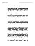
Figure 2.2

Figure 2.2 shows that if economies of scale exist throughout the relevant range of output, large firms can produce output at a lower cost than can smaller firms. Suppose, for example that all of the firms have the average total cost curve ATCo. If one of them becomes larger than the others and can produce output at a lower cost per unit (as illustrated by the curve ATC'), the larger firm can sell its output at a lower price P' at which smaller firms will experience economic losses since it cannot recover its cost (Note that at ...

This is a preview of the whole essay

Figure 2.2

In this situation, the smaller firms will eventually be forced to either leave the industry or merge with other firms to become at least as large as the current largest firm. As firms keep growing (either through internal expansion or by buying up smaller firms), their average costs continue to decline. Smaller firms continue to disappear until eventually only one large firm remains, which is the natural monopolist. When it becomes a natural monopoly, than it can charge back the price as illustrated in Figure 2.1.

As you can immediately notice that is much higher than MC, representing a substantial profit margin, you may then jump to the conclusion that consumer is better off when under competition where P=MC with a higher level of output. However, I will leave this for discussion in the later part of the paper. For the time being, we will take it as it is. The fact that natural monopoly is one form of monopoly indicates that we should spend some time in understanding what it is.

III. MONOPOLY VERSUS COMPETITION

Monopoly

A monopoly is a situation where there is only one seller in the market. A firm under perfect competition is often regarded as a price taker because it has no effect on the market demand and price by making decision. It takes the market prevailing price as given and can only decide on what quantity to produce. However, a monopolist's demand is in fact the market demand, and hence the monopolist can set its own price. Then a question arises – what makes a monopoly a monopoly?

There are several possible reasons for the existence of monopolies, each of which creates what we call “barrier to entry” which makes the market closed in some way.

First, a firm may control the entire supply of a basic input that is needed to produce a certain product. For example, the Aluminum Company of America (Alcoa) controlled the world’s bauxite which is an essential raw material in the production of aluminum prior to World War II.

Second, the industry may be a natural monopoly as we mentioned a while ago. The natural monopoly’s production exhibits decreasing average cost (economies of scale) in the output range that would meet the entire market demand at a profitable price and it is desirable to have only one firm to minimise the production cost. Public utilities are often examples of natural monopolies.

Third, monopolies may be created through laws and government regulations. Sometimes the government may make it illegal for firms other than the existing one to enter into a market or it may require the firms to obtain some certificates or license in order to do so. However, obtaining this approval is often very difficult, thus deterring others from entering the market. One case is the legal protection for patents. The purpose of this is to provide incentives for innovation.

Comparison of Perfect Competition and Monopoly

As we can see from the previous diagrams that monopoly price is higher than marginal cost, this creates a dead-weight loss. (Recall that under perfect competition, price equals marginal cost). Figure 2.3 (a) illustrates the consumer and producer surplus that is received in a perfectly competitive market. Figure 2.3 (b) illustrates the loss in consumer and producer surplus that results when a perfectly competitive industry is replaced by a monopoly. The area that is between the supply curve and the price line measures producer surplus (orange shade). The area between the price line and the demand curve measures consumer surplus (yellow shade).

Now, Figure 2.3 (b) shows us what happens when perfect competition is replaced by monopoly. The introduction of a monopoly firm causes the price to rise from P(pc) to P(m) while the quantity of output falls from Q(pc) to Q(m). The higher price and reduced quantity in the monopoly industry causes consumer surplus to shrink to ACP(m) (yellow shade) and the producer gain additional surplus from the part P(m)CEP(pc) which is being transferred from consumer surplus under competition. The net cost to society is equal to the blue shaded triangle CBF. This net cost of a monopoly is called deadweight loss. It is a measure of the loss of consumer and producer surplus that results from the lower level of production that occurs in a monopoly industry.

Figure 2.3

However, I would say that the model above over-generalises the whole situation for simplicity’s sake. In real life situation, the threat of potential competition may encourage monopoly firms to produce more output at a lower price (to deter potential entry) than the model presented above suggests. This heavily relies on the effectiveness of the barriers to entry. Fear of government intervention (in the form of price regulation or antitrust action as in the USA) may also keep prices lower in a monopoly industry than would otherwise be expected. Either case would reduce the actual deadweight loss or economic welfare (as some may call it) as a result of the existence of a monopoly.

One deficiency of this diagram is that it assumes that MC (as in Figure 2.3 a) is the same for both perfect competition and monopoly situation but it is not necessarily to be the case. While competitive firms may produce more output than a monopoly firm with the same cost curves, a large monopoly firm produces output at a lower cost than could smaller firms when economies of scale are present, meaning that they might have different marginal cost curves. If we took this into consideration, the deadweight loss might have been reduced.

On the other hand, deadweight loss may understate the cost of monopoly as a result of either X-inefficiency or rent-seeking behavior. As introduced by H. Leibenstein, the X-inefficiency is the theory of inefficiency generated from non-competition and can be applied to the monopolies if they have less incentive to produce output in a least-cost manner since they are not threatened with competitive pressures. Firms are involved in rent-seeking behavior when they allocate resources in hiring lawyers, lobbyists, etc. in an attempt to receive governmentally granted monopoly power. These “rents” are uncompensated, yet divert resources away from productive activity, thus being considered as socially unproductive.

IV. REGULATION OF NATURAL MONOPOLY

Until this point it is clear that monopolies can be considered as inefficient because they produce a lower output and charge a higher price than competitive firms would and that they incur deadweight loss. Therefore, from consumers’ point of view, their welfare is not maximised as they pay higher price for goods (if they can get any since the quantity is reduced). This gives room for government to step in. Government regulates monopolies mainly for: (a) to make the monopoly more efficient (b) to maximise consumer welfare. It can achieve these by requiring the firm to produce more efficiently and to produce more output so that price is equal to MC. However, at point P=MC, MC>MR and the firm loses money. Figure 2.4 illustrates alternative regulatory strategies in such an industry. If the government keeps its hand off, the monopoly will maximise its profits by producing at Q(m) and charge P(m). Suppose now the government attempts to intervene by setting P=MC. This would occur at P(mc)Q(mc). The average cost curve declines everywhere, hence marginal costs must be less than average costs. Thus, if the price equals marginal costs, the price will be less than average total costs and the monopoly firm will experience economic losses and the firm will not stay in the industry unless it receives government subsidies in the production of this good in the long run. In many case we will see that the government would provide a subsidy to make up the difference between price and marginal revenue, but that is expensive to taxpayers, who, in order words, are the final consumers.

Figure 2.4

Therefore, a more common and desirable strategy is to allow the owners of the monopoly receive only a fair or normal rate of return instead of monopoly profits. This could be done through a price set at P(f). At this price, it would be optimal for the firm to produce Q(f) units of output and there would be no incentive for this firm to leave the industry. This is the common pricing strategy that regulators use in establishing prices for utilities, cable services, and the prices of other services produced in regulated monopoly markets.

This strategy would allow firm a fair (normal) rate of return and more output than the MR=MC level of output, although still less than the optimum efficiency of P=MC.

V. CONCLUSION

In a monopoly situation, it is said that firm owners expend consumer welfare for their own profits as well as creating deadweight loss. However, there are situations where monopoly operation is inevitable as it is the most economical way of produce certain products and that the size of deadweight loss is difficult to be measure accurately for reasons mentioned in this paper. Therefore, there is not an absolute yes or no to the idea that competition is always preferable to monopoly. However, one possible way to ensure that consumer welfare is being protected from extreme monopoly pricing lies on the government’s hand. It plays a role in balancing consumer welfare with cost-effective production in a monopoly. We have seen that government could either set P=MC but subsidise the firm in the long run to keep it in the industry or set P=AC so that it main zero economic profit. Both ways seem reasonable but subsidising firms may represent higher burden on the taxpayers who are in fact the consumers, therefore I think that the second way is more justified and fair in terms of maximising consumer welfare.

Although this paper set out quite some justifications on the size of the deadweight loss, I have to admit that, as previously mentioned, the ignorance of the fact that marginal cost curves under perfect competition and monopoly may not be the same and that other elements may affect the size of the deadweight loss such as the effectiveness of barriers to entry and government intervention to simplify the model. However, I think the main purpose of comparing perfect competition and monopoly in general and explaining consumer welfare in both cases can somehow be achieved.

VI. REFERENCE

ESTRIN, S., LAIDER, D., (1995), Introduction to Microeconomics, 4th Edition, New Jersey: Prentice-Hall, Inc.
LEIBENSTEIN, H., (1980), Inflation, Income Distribution and X-efficiency Theory, Barnes & Noble Books-Imports
MILLER, R.L., (2000), Economics Today, 10th Edition, New York: Addison-Wesley Publishing Company Inc.
PINDYCK, R.S., RUBINFELD, D.L., (2001) Microeconomics, 5th Edition, New Jersey: Prentice-Hall, Inc.