Industry MR
0 Q1 Q
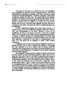
If all the components concur on the cartel price, they may after that, contend against each other by means of non-price competition, with the purpose of gaining as big a share of resulting sales (Q1) as they can.
Alternatively, the cartel elements may in a way consent to separate the market between them. In such a case, each member would be given a quota. The calculation of all the quotas must be equivalent to Q1. If the quotas went above Q1, either there would be output unsold if price remained permanent at P1, or the price would go down. The cartel will come to a decision for the level of each person’s quota by separating the market among the members in keeping with their existing market share. This is believed to be the most ‘fair’ clarification.
Occasionally open collusion may be against the law. Then firms either break the law or get round it. On the other hand, firms may stay contained by the law, but still tacitly collude by watching each other’s prices and keeping theirs alike.
There are two modes of tacit collusion, the ‘price leadership’ and the ‘rules of thumb’. Taking into account price leadership, we have to pass on to its two forms; the dominant firm price leadership and the barometric firm price leadership. In the dominant firm price leadership, the leader has to place a price, in which his profits will be maximized, where its marginal revenue is equivalent to its marginal cost.
Figure 2, shows the total market demand curve. The supply curve of all followers is also established. These firms confess the price as decided, just in this case it is the price placed by the leader, and consequently their mutual supply curve is in essence the sum of their MC curves. The leaders demand curve can be seen as that segment of market demand vacant by the other firms. In other words, it is market demand minus other firms’ supply. At P1, the other firms talk into the intact market demand, and as a result, the demand for the leader is zero (point a). At P2, the other firms’ supply is zero, and thus the leader deal with the full market demand (point b). The leader’s demand curve consequently gets points a and b along.
Figure 2
Division of the market between leader and followers
£ S all other firms
P1 a
D market
D leader
P2 b
0 Q
Figure 3 shows that the leader’s profit will be maximized, at the point that its marginal cost equals its marginal revenue. Actually, this diagram is the same as figure 2, but with the accumulation of MC and MR curves for the leader. The leader’s marginal cost equals its marginal revenue at an output of QL, (giving a point l on its demand curve). The leader thus sets a price of PL, which the other firms then duly follow. Then supply QF (i.e. at point f of their supply curve). Total market demand at PL is QT (i.e. point t on the market demand curve), which must add up to the output of both leader and followers (i.e. QL+QF).
Figure 3
Determination of price and output
£
MC leader S all other firms
l
PL f t
D market
D leader
MR leader
0 QL QF QT Q
Actually, though, it is complicated for the leader to be relevant to this theory. The leader’s demand and MR curves rely on the followers’ supply curve, which is something that the leader will get roughly impractical to approximate with any quantity of correctness. For this reason, the leader will have to make a cruel assumption of what is profit – maximizing price and output will be, and simply prefer that.
Nonetheless, there is a simpler model, which conserves a constant market share. It makes such a supposition since it as well presumes that all other firms will go after its price up and down. On the other hand, this simpler model cannot be carried out since the statement that the followers will yearn for to preserve a constant market share, comprises a problem. Related to the dominant firm price leadership is the barometric firm price leadership in which the firm is not dominating the industry but is taken as a barometer to the others. Therefore, in accordance with the barometric firm’s actions, the others will react in the same way.
With the intention of having an conventional leader, we can have an reputable set of effortless ‘rules of thumb’ that all go after. These rules assist to put a stop to an eruption of competition and thus, lend a hand to retain profits in the long term. Such rules are the ‘average cost pricing’ and the ‘price benchmarks’. ‘Rules of thumb’ can furthermore be functional to presenting or to the design of the product.
There are more than a few factors that errand collusion. So, if:
- There is a small number of, eminent to each other firms,
- They are not enigmatic about costs and production techniques,
- They have comparable production methods and average costs,
- They produce related products,
- There is a dominant firm,
- There are ‘barriers to entry’,
- The market is constant,
- There are no government measures to hold back collusion,
it would be easier for the firms to collude.
When the above factors do not exist it is possible price competition to happen. In such a case, firms do not collude, but struggle each other and at last, the consequence is a ‘price war’, which means that the price would then decrease. In such a case, firms have to prefer the suitable ‘strategy’ that will excellent be successful in getting the better off their challengers.
In proportion to the economists, the best strategy is the game theory. The simplest model is when there are just two firms with indistinguishable costs, products and demand. Supposing that there are two firms X and Y that they have both set their price to £2 that they are each making a profit of £10 million, giving a total industry profit of £20 million. If they both reduce their price to £1.80, they have to consider what the rival one will do. Table 1 demonstrates usual profits they could each make in any case:
Table 1
PROFITS FOR FIRMS X AND Y AT DIFFERENT PRICES
X’s price
£2 £1.80
£2
Y’s price
£1.80
The guiding principle of accepting the safer strategy is called maximin; the firm will go for the alternative that it will maximize it minimum profit. A substitute strategy is notorious as maximax; going for the maximum profit. Taken for established that in this ‘game’ maximax and maximin lead to the same strategy, this is known as a dominant strategy game. with the exception of that, there can be more complex ‘games’ within more than two firms, where firms go on a negotiation strategy. Occasionally, firms may compete hard for a time and then become conscious that nobody is winning. At that point they may set up to collude and increase prices. Consequently, competition may stop working again.
The benefit of the game theory is that the firm does not necessitate to be acquainted with which retort its opponent will make. As a result, such a loom is merely constructive in moderately plain cases.
On the other hand, the most well known theory in oligopoly is the kinked demand curve, which makes clear how prices can remain constant, even if there is no collusion. This theory is rooted in two unbalanced statements:
- If an oligopolist curtails its price, its opponents will pursue and
- If an oligopolist inflates its price, its opponents will keep their prices the unchanged.
On these statement, each oligopolist will facade a demand curve that is kinked at the existing price and output, as it is illustrated in figure 4.
Figure 4
Kinked demand for a firm under oligopoly
£
P1
D
0 Q1 Q
An increase in price will bring about a descend in sales; the curve is comparatively elastic above the kink. On the contrary, a decrease in price will set in motion a diffident augment in sales; the curve is comparatively inelastic below the kink. This price constancy can be properly exposed by drawing the firm’s marginal revenue curve, which is illustrated in figure 5.
Figure 5
Stable price under conditions of a kinked demand curve
£
MC2
MC1
P1
a
D=AR
b
0
Q1 MR Q
“To see how it is done, imagine dividing the diagram into two parts either side of Q1. at quantities less than Q1, the MR curve will correspond to the shallow part of the AR curve. At quantities greater than Q1, the MR curve will correspond to the steep part of the AR curve. To see how this part of the MR curve is constructed, imagine extending the steep part of the AR curve back to the vertical axis. This is the corresponding MR curve are shown by the dotted lines. It is obvious that there will be a gap between points a and b. in other words, there is a vertical section of the MR curve between these two points. Profits are maximized where MC=MR. Thus, if the MC curve lies anywhere between MC1 and MC2, the profit maximizing price and output will be P1 and Q1. Thus, prices will remain stable even with a considerable change in costs”. (John Sloman, economics, fourth edition, page 189).
Nonetheless, the model has besides two precincts:
Price constancy may be because of supplementary factors; consequently it is no evidence of the correctness of the model,
even though the model can be of assistance to clarify price constancy, it does not put in plain words how prices are set in the first place.
Drawing a conclusion, even if there are quite many models, which give the impression in some way to foretell how the firms, in oligopoly markets, will act in any alteration of price, all of them have a number of chief limitations. Those limitations give us a testimony that there is no theory envisaging firms’ behaviour in oligopoly markets.