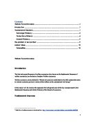
If we keep drawing indifference curves through points inside the new lens-shaped area, we will get to a point where there is no more Pareto improvement or in other words a point where there are no more trades preferred by both person A and person B. This point is known as a Pareto efficient allocation and at this point individual A and individual B’s indifference curves are tangential.
The set of allocations where by the indifference curves of individual A and that of individual B are tangential can be connected by a line called the contract curve (illustrated below). Any point off the contract curve means that the marginal rate of substitution of A and B differ hence meaning that there is an opportunity for Pareto improvement.
This means that for any point on the contract curve MRSA1,2 = MRSB1,2
Additionally we know that individuals seek to maximize utility their subject to their budget constraint hence giving:
MRSA1, 2 = P1/P2 and MRSB1, 2 = P1/P2
Therefore we have MRSA1, 2 = MRSB1, 2 = P1/P2
This is the condition for exchange efficiency.
Xb1
B
Xb2
Xa1 good1
Production efficiency
So far we have analysed a pure exchange economy that is one where no production occurs. To meet the second condition required for the first theorem we must analyse an economy where production occurs.
This time we have two firms A and B that employ two factors of production labor L and capital K to produce outputs of two different goods (good 1 and 2). Additionally instead of indifference curves we have isoquants which represent different combinations of labor and capital that give the same output of good 1 or 2.
The slope of the isoquant curve measures the Marginal rate of technical substitution (MRTS). The MRTS shows how much one factor of production must be increased by in order to compensate for a decrease in another factor so that total output is the same. Another way of defining MRTS is by saying the marginal physical product of capital used to produce good 1 divided by the marginal physical product of labor.
Here MRTS1kl = -ΔL/ΔK = MPPK/MPPL where MPP stands for marginal physical product
The red line is the isocost line which shows the total cost of production. The slope of the isocost line therefore is equal to –PL/PK. In order to minimize cost the firm must produce where the isoquant is tangential to the isocost curve ( point E).
Here MRTS1= -PL/PK
If we combine firm A and B equilibria’s using an edgeworth box we get:
XbL
2
XbK
XaL L
As analysed previously in our analysis of exchange efficiency there will be points where if the producers of good one and good two were to trade voluntarily, there is the possibility of a Pareto improvement. Such a point is illustrated above at point E and a Pareto improvement can be obtained by moving to point N.
Production efficiency would be attained when all possible Pareto improvements have been exhausted (Illustrated below).
Xb1
B
Xb2
Xa1 good1
At this point the isoquants of the two firms are tangential. We know that the slope of isoquant measures MRTSKL.
This means that the MRTS1kl = MRTS2kl
Additionally we know that firms seek to individually maximise profits by minimising cost therefore
MRTS1kl = MRTS2kl = -PL/PK
This is the condition for production efficiency.
Additionally we can plot all the points on the contract curve to construct a production possibility frontier (PPF).
Illustrated PPF
Good 1
All the points on the PPF represent the maximum amount of good one that can be produced relative to good 2. Any point outside PPF is unattainable and any point inside are inefficient.
Overall Efficiency
Overall efficiency is achieved when both production and exchange efficiency are attained simultaneously. For this to happen MRS must equal MRTS and this would occur when the PPF is just tangential to the consumers indifference curve.
One of the major shortcomings of the first theorem is that there is no unique optimum. Anywhere on the ppf is optimal.
The problem of second Best
Attaining a Pareto optimal state would be desirable because it would mean that resources in the economy are allocated in the most efficient way possible given the demand of society. The first theorem gives and argument for free-markets1
However, there are factors such as monopolistic power and externalities (market failure) which make obtaining the conditions required for Pareto efficiency impractical. So given that the first best condition cannot be achieved should we then put in place a system whereby a second best allocation based on the rules of first best is achieved? ‘In principle this can be done via taxation/subsidies such that all necessary conditions can be fulfilled and a first best can be achieved’.
However according to the theory of second best the answer is no. According to the theory of second best given that there are constraints that violate the some of the conditions necessary for Pareto optimality, then meeting the other conditions that are not violated is not desired and may actually decrease economic efficiency .
The implication of the theory of second best is that where first theorem stated there is no efficiency role for government, ‘the second theorem argues that all possible efficient allocations can be attained given an appropriate initial allocation of goods’.
Market failure
A market failure is a case in which a market fails to efficiently provide or allocate goods and services. This arises because some of the conditions necessary for Pareto optimality are not met. I will examine how market failure arises in and Externalities in Monopoly and possible ways in which these failures can be overcome
Externalities
An externality can be defined as the effect of one party’s economic activities on another party that is not taken into account by the price system.
To illustrate this we will take the example of negative Externalities. Negative Externalities is the separation of social cost of and economic activity from the private cost.
Imagine two firms (A and B) firm A is a company that produces shoes and is situated near an airport. Firm B is the airline company who owns the airport. The ability of firm A to produce shoes is affected by the level of noise pollution from the airport caused by Firm B. the workers at firm A cannot concentrate on the task of producing shoes because of the level of noise pollution. Therefore the noise pollution caused by firm B has an external effect on the production of shoes.
However because firm B does not have to pay for the noise pollution the social cost of their noise pollution is not taken into account by the price.
The social cost in this case can be defined as ‘costs of production that include both input costs and the costs of externalities that production by cause’. Because firm B is not taking into account the cost of their externalities they are only paying for the cost of their inputs i.e. private cost. This means that firm B can produce more than if they had taken into account social costs hence meaning they are likely to make more profits. This means there is a market price which does not take into consideration the social cost and therefore leads to a misallocation of resources (market failure).
This scenario can be illustrated as follows
p
q1
In a perfectly competitive market where there are no externalities price would be equal to marginal private cost. Therefore at a price of P a quantity of Q1 would be produced. This means that all of the cost of production is incorporated by the private marginal cost curve. However because of externalities we have to consider the marginal social cost of production of firm B
Q2 Q1
As you can see the social marginal cost exceeds the marginal private cost of firm B. The vertical gap between the MPC and MSC represents the noise pollution suffered by Firm A (the shoe maker). Taking into account the MSC curve we now we have a new equilibrium position p2 and a new output level Q2. Q2 is the best price allocation of as it takes into account both private and social costs of production. However due to market failure we are producing Q1 which is a misallocation of resources as at this point the social marginal cost of the production of firm B exceeds the price which people are willing to pay for the level of output. Therefore there is an overproduction (inefficiency) by firm B at this point. This can be represented on the diagram by the area shaded red.
Q2 Q1
One way those economists overcome the market failure caused by such an externality is by imposing Pigou taxation. The Pigou tax works by raising the cost of production of Firm B this would in turn cause the marginal private cost curve to shift to the left up until it reaches the marginal social cost curve. This means that price will go up from P1 (market price) to P2 and the quantity of output will go down from Q1 to Q2 which we identified as the social optimum allocation hence overcoming the market failure caused by the negative externality.
P1
Q2 Q1
Another cause of market failure is non- competitive behaviour. This is because one of main conditions required for Pareto efficiency is that price is equal marginal cost (MC) meaning that all the firms in the industry are price takers and therefore have no say in determining the market price. However in the real world we have instances where due to insufficient competition that some firms can determine their own prices and hence can operate where price is greater than MC One such case is a monopoly.
p2
P1
MR
Q2 Q1
From the graph above we can see that where P=MC we would have a price of p1 and an output of p2. However because a monopolistic firm appreciates that it can influence market prices due to entry barriers and insufficient competition then the firm will opt to produce at a price of p2 and a quantity of q2. This means that under monopolists price is higher (p2>p1) and quantity is lower (q1>q2).
Inefficiency in monopoly
We can see from the graph that for quantities q2 to q1 P>MC. This means that for all output levels between q2 and q1 consumers are willing to pay more for a unit than it costs to produce it. Hence there is the possibility of a Pareto improvement. If the firm were to produce this extra unit and sell it at any price lower than p2 but greater than MC both consumer and producer are made better off hence a Pareto improvement has occurred. The problem however is that monopolist firms can’t produce at a price lower than the market price as it has to take into account the effect of increasing output on the revenue received from the inframarginal units. This means that in order to sell an additional unit at less than market price it would have to lower the price of all of its other units it currently sells.
Deadweight loss
p2
P1
MR
Q2 Q1
So what we have is an area on are graph where consumers are willing to pay more for a unit of output than it costs to produce it however this unit is not being produced therefore it is inefficient as we know a Pareto improvement can take place. This area is shaded in red above.
Deadweight loss
p2
P1
MR
Q2 Q1
One solution to this problem is regulation. If the monopolistic firm can be forced to sell where price is equal to marginal cost then the deadweight loss is minimised. However this would need to the regulator to identify the marginal cost of the firm and if this must be attained by the firm itself they might say that their marginal cost is much higher say at MC2 than what it actually is and hence they end up paying the same monopolistic price of P2.
Bibliography
Definition of welfare economics obtained from
2Marginal rate of substitution is the extra amount of one needed to compensate a for a decrease in the amount of another product definition from
3 Edgeworth box is diagram devised by F. Y. Edgeworth, in the form of a box which plots the of two individuals or relative to the or of two .
4 In principle this can be done via taxation/subsidies such that all necessary conditions can be fulfilled and a first best can be achieved’Extract from book called Welfare economics-introduction to basic concepts by Yew kwang ng 1979
6 Extract from Perloff ,microeconomics 4th edition page 318
7 A situation in which a all or nearly all of the for a given type of or .
Definition of welfare economics obtained from
Marginal rate of substitution is the extra amount of one needed to compensate a for a decrease in the amount of another product
Edgeworth box is diagram devised by F. Y. Edgeworth, in the form of a box which plots the of two individuals or relative to the or of two .
Xa represents A’s consumption and Xb represents B consumption e.g Xa1 +Xb1 = total amount of good 1 available
Extract from book called Welfare economics-introduction to basic concepts by Yew kwang ng 1979
Extract from Perloff ,microeconomics 4th edition page 318
A situation in which a all or nearly all of the for a given type of or .