(7)
The second method, “on/off” control, focuses on the extremes of desired performance. The initial water temperature has two settings: the low or “off” setting and the high or “on” setting. When the average temperature becomes higher than desired, the initial temperature is set to the “off” setting. When the average temperature drops too low, the initial temperature is increased to the “on” setting.
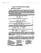
ε: Emissivity mw: Mass flow rate T∞: Air temperature
σ: Stefan-Boltzmann P*: Equivalent channel width Tout: Out-going temperature
cw: Specific heat of water Q: Total heat rate TP: Patient temperature
hA: Water-skin heat transfer coef R: Thermal resistance Tw: Water temperature
hB: Skin-air heat transfer coef T: Time Twall: Room temperature
KP: Proportionality constant Td: Target temperature x: Distance
Mw: Total mass Tin: Initial Temperature
- PROBLEM STATEMENT & RESULTS
Part I: Steady-State Simulation
The first half of this project simulated the heat transfer of a hypothermia bed using a steady-state simulation, a scenario in which all heat transferred to the patient is in turn transferred to the environment through convection and radiation. First, a 3D-plot of the mass velocity and initial temperature vs. change in temperature was programmed. The resulting Figure 1 shows how ΔT increases linearly with mv and exponentially with Tin. From the figure, values for mv and Tin can be estimated at 0.02 kg/s and 40°C, respectively.
A plot of Tw vs. position was then made using a simple Euler progression and Equation 1. This plot is shown in Figure 2. From this method, the temperature of water leaving the system is found to be 313.5 K.
The mean temperature of the water was found using the equation
(8)
where T(x) is from Equation 2. Evaluating this integral from L=0 to L=2m, Tw is found to be 314.85 K.
The heat transfer rate was calculated directly from Equation 3. Here, Tout was determined using the Euler’s method employed in plotting T vs. position. The resulting MATLAB script produced an output of 302.72 J/s.
The steady-state quality of this simulation is due to the equal transfer of heat from the bed to the patient and from the patient to the surroundings through convection, conduction, and radiation. Thus, Equation 3 can be set equal to Equation 4, resulting in a fourth-degree equation for the surrounding temperature. Using the “roots” command, MATLAB was used to solve this resulting polynomial, producing one real solution of 296 K. (See Appendix A)
Finally, with a Tin of 42°C, mv is to be determined in order to maintain the patient at 37°C. By substituting Equation 2 into Equation 3, and maintaining the previously found value of Q, a plot of mv vs. ΔT is made. From this plot, the value of mv is estimated as 0.0337 kg/s. Evaluating Equation 3 for this mv, the corresponding Tin is calculated to be 313.85 K (See Appendix A)
Part II: Time-Dependent Control
The time-dependent control portion of this project dealt extensively with basic, first-order differential equations. The first problem asked that, for a given initial temperature Tw(0)=39.5°C and Tin=40°C, the steady state value of Tw be determined. Equation 6 was solved through separation and integration, resulting in the following equation of Tw(t):
(9)
Applying this equation to an array of Tin and plotting vs. t results in Figure 3. From this chart, Tw can be seen to approach 311.5 K asymptotically, making this value the steady state value of Tw. The time constant, τ, can be determined from the exponential component of Equation 9. Since
(8)
then τ=1/(A+B).
The second portion dealt with a proportional control system, asking for a proportionality constant, KP, for a system with time constant τ/10 and target value Td=38.5°C. Substituting Equation 7 for Tin in Equation 9, separating the variables, and integrating as before, the following solution for Tw(t) results:
(10)
Setting τ1 from the previous portion equal to the new τ2, KP can be calculated as 17.999. (See Appendix B) It should also be noted that as t approaches infinity, the second half of the sum in Tw(t) approaches zero and thus Tw(t) approaches 295.8495 K. For this reason, Tw will not reach Td under the specified conditions.
The final portion of the time-dependent control phase employed an “on/off” control system. Here, if Tw dropped below 38.25°C, Tin was switched to 42°C, while if Tw rose above 38.75°C, Tin switched to 34C. This function was coded in MATLAB using a series of “if” statements, as well as Euler’s method. (See Appendix B) The resulting oscillating plot is shown in Figure 4. From this plot, the number of oscillations (i.e., number of peaks or troughs in the wave pattern) may be simply counted over a measured length of time, resulting in the frequency of oscillation of Tw. In this graph, thirteen oscillations occurred over a 10 second interval, illustrating the function’s frequency to be 1.3 Hz.
- CONCLUSION
Through this project, the nature of fluid/thermal systems has become apparent and their association with differential equations made obvious. In addition, several methods for controlling these fluid systems: proportional control and on/off control, have been investigated. Tying all these concepts together was their interrelated use in a real-life application, namely a hypothermia bed.
APPENDIX A:
SELECTED STEADY-STATE PROBLEM CODES
clear
Tp = 310; %Temperature of person (C)
P = 0.12; %Total width (m)
hA = 260; %Water-Skin heat transfer coeffecient (W/m^2*K)
hB = 6; %Skin-Air heat transfer coefficient (W/m^2*K)
cw = 4180; %Specific heat of water (J/kg*K)
epsilon = 0.95; %Emissivity
sigma = 5.67E-8; %Stefan-Boltzmann constant (W/m^2*K^4)
e = 2.71828; %Natural base
mw = 0.02411; %Mass flow rate (kg/s)
Tin = 316.5; %Flow in temperature (K)
L=2; %Length of pipe (m)
i=1; %Initialize counter
x(1)=0; %Set initial position (m)
Told(1)=Tin; %Set initial temperature (K)
dx = .01; %Set change in position
A=1.8; %Surface are of heat transfer (m^2)
while x(i) <= 2.01
dtdx=(-(hA*P)/(mw*cw))*(Told(i)-Tp); %Calculate change temperature/change position
Tnew(i) = Told(i) + dtdx*dx; %Calculate temperature after position change
Told(i+1)=Tnew(i); %Set final temperature equal to initial temperature of next stage
x(i+1)=x(i)+dx; %Phase shift position
i = i + 1; %Increase counter
end
Q = (mw*cw*(Tin-Told(i))) %Total heat rate (J/s)
C = [-epsilon*sigma*A 0 0 -hB*A epsilon*sigma*A*(Tp^4)+hB*A*Tp-Q] %Create polynomial matrix
roots(C) %Find zeros of polynomial matrix
============================================================================
for mw=(.001:.00001:.1)
F(i)= ((mw*cw*(Tin-(Tp+(Tin-Tp)*e.^((((-hA*P)/(mw*cw)))*2))))-Q); %Write to heat rate matrix
p(i)=mw; %Write to mw matrix
i = i + 1; %Increase counter
end
plot(p,F) %Plot
xlabel('mw (kg/s)');
ylabel('Delta T (K)');
axis([.03 .035 -5 5])
grid on
mw=0.0337 %mw determined by inspection
Tout = Tp + (Tin-Tp)*e.^((-2*hA*P)/(mw*cw)) %Calculate corresponding Tout
APPENDIX B:
SELECTED TIME-DEPENDENT PROBLEM CODES
clear
Tp=310; %Temperature of person (K)
L=2; %Length of Bed (m)
cw=4180; %Specific heat of water (J/kg*K)
mw=0.4785; %Mass flow rate (kg/s)
Mw=2; %Total mass (kg)
R=2.5e-4; %Thermal resistance
T0=312.5; %Initial temperature (K)
Tin=313; %Initial temperature (K)
Td=311.5; %Target temperature (K)
e = 2.71828; %Natural base
i=1; %Initialize counter
A=2*mw/Mw; %Calculate A
B=1/(Mw*cw*R); %Calculate B
Kp=(9*A + 9*B)/A %Calculate proportionality factor
for t=[1:.1:20]
Tw(i)=(A*Kp*Td+B*Tp)/(A+A*Kp+B) + (T0-(A*Kp*Td+B*Td)/(A+A*Kp+B))*e.^(-(A+A*Kp+B)*t);
ti(i)=t;
i=i+1;
end
plot(ti,Tw)
grid on
============================================================================
for t=[0:.01:10]
dTw(i) = (-A*(Tw(i)-Tin)-B*(Tw(i)-Tp))*dt;
Tw(i+1)= Tw(i) + dTw(i);
if Tw(i)>=311.75
Tin=TL;
ti(i+1)=ti(i)+dt;
i=i+1;
elseif Tw(i)<=311.25
Tin=TU;
ti(i+1)=ti(i)+dt;
i=i+1;
else
Tin=Tin;
ti(i+1)=ti(i)+dt;
i=i+1;
end
end
plot(ti,Tw)