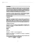
Firgure 1.Number of people residual plot Firgure 1.Number of rooms residual plot
Firgure 1.Number of income residual plot
Residual plots of income, number of rooms and number of people in a household against the predicted electricity expenditure show that there is little indication of heteroscedaticity. The variances just vary in certain ranges and do not make any patterns. In the graph of “people”, an oval shape can be imagined; or a wave shape may be compared to the residual plot in graph of rooms. However, there is no concrete evidence to indicate they are a result of heteroscedasticity. Some outliers can be the reason for those unclear shapes.
In summary, it is reasonable to conclude that the full data are fair, unbiased and satisfactory to the CLRM assumptions.
The report is overall well written. It follows a logic progression. The following parts are to be analysed.
a. Executive summary:
This part of the report is quite concise and appropriate. The point form is used to reduce the length but increase clarity. Non-technical language supports a more understandable report for everyone; this is successful as it aims at achieving reader’s understanding without technique “babble”. Moreover, all objectives of the projects and main results are clearly outlined in this part.
b. Introduction:
The advantages of conciseness and non-technical language can be found once again in this part. Just by a short paragraph, the introduction covers all main points of the report. In addition, the content is in more ordered fashion, i.e. it starts from the aim, then data collection, data analysis and some brief conclusions. Although the introduction basically repeats the executive summary, it differs in regards of written structure. Bullet points are replaced by paragraph.
c. Data description
This part of the paper is clear, concise but incomplete. Indeed, the sample is well described of what it is and how it was collected, e.g. forms of the data, number of the sample, and number of audited households are listed. However, there is no mention of other variables collected out of the four variables named and why those variables are omitted. Seriously, no summary statistics of any variable is provided, this leads to a lack of key feature descriptions of data. Therefore, errors, outliers or other problems of the data can not be examined.
Data and their features should be presented in an appendix.
d. The regression model
The advantage of conciseness actually has a counter effect on this part. It is too much concise and in severe lack of technical language and details. The report says very little about building the model and underlying assumptions. In this very important part of the project where is a fundament for every later conclusion, any related reason should be fully presented and any necessary technique should be applied. Particularly, when econometrics has been chosen to be the media of analyzing the data, the work must have been done in logic order under requirements of a model regression building in econometrics.
The paper does not give any reason for choosing the model or omitting variables. No explanation and no evidence are stated to prove that the model is not misspecified. Depending on data and purpose of report, etc, a model can be linear, quadratic or log forms. There should be a discussion about this or at least a review of the similar paper to know what variables should be included in the model. Indeed, there are a variety of methods to improve the model, e.g. variables can be transformed to log, interaction variables can be added, etc. However, none of them is presented including some basic diagnostic tests such as tests of heteroscedasticity, autocorrelation, etc to give the model statistical credibility.
Interpretation is inadequate and not justified formally by appropriate statistic tests or economic theories. E.g. in the interpretation of “significance” of the model (3), coefficients of ROOMNO (5.4) and DAUD (-2.2) without any explanation that can mathematically results to the conclusion of a better model. In addition, the conclusions of R2 and ROOMNO are not supported by any statistics.
Another shortcoming of the interpretation is that meanings of those given statistics are not interpreted, i.e. relationships between variables are not expressed in words, that may cause difficulties in understanding for many readers. It is easy to eliminate that problem by adding some simple statements of the relationship, e.g. on average, for an additional unit of rooms a household has, its electricity expenditure increases by 71.4 units (this is for model (3)).
Finally, no economic theory is discussed behind the model. Some of them may be very helpful such as consumer’s utility or savings behaviours. There is, hence, little priori expectation and basic theory to check with the results. This lack of reasoning would reduce the persuasiveness of the model.
e. Conclusion
The paper jumps straight to a brief and incomplete conclusion. No attempt is made to mention the data flaws and modeling problems, i.e. as there are always gaps between data analysis and the conclusions, the conclusions have no clue for itself. The relationship between the conclusion and the previous parts is ignored. Therefore, people may not know why the audit program is concluded to be effective and how effective it is.
Moreover, no discussion of implications and areas for further study to be done. The data is not available for replication, no appendix of calculation or regression analysis and no reference are given. This is a severe mistake of an academic report.
ELEXP = β1 + β2 PEOPLE + β3ROOMNO + β4INCOME + β5DAUD + β6 DGAS +
Β7DAUAD*DGAS + u
We start with a large model, ie. we are trying to cover all possible effects, then may drop some inappropriate variables.
a. Why choose the model
Linear model is chosen since it can best satisfy the purpose of the project which is to determine the effectiveness of audit programs on energy savings. Linear form gives direct effects while other forms may focus on other aspects, e.g. log-log represents elasticity, etc.
Intercept: As discussed in part 2.b, intercept should only be dropped if we have a significant expectation of a non-constant model. Indeed, omitting intercept may cause many problems such as inaccurate R2, insignificance of parameters, etc. Therefore, it is safe to keep the intercept until there is a concrete theory suggesting no do so.
Number of rooms and people: These have positive relationships with electric expenditure. On average, it’s quite clear that the larger the numbers of rooms and people the higher the electricity expenditure.
Income: Although income, according to Keynes, does not contribute its full increase to expenditure (since there is an increase in savings as income increases), income still has a positive impact on electric expenditure. When income rises, people have more money to afford the increase in electricity expenditure.
DAUD: is a compulsory in the model. Whatever the significance is, we still have to keep DAUD for purpose of the model.
DGAS: may attract concerns about its substitution effects for electricity. We expect that if DGAS = 1 household’s electricity expenditure is reduced by a certain amount.
DAUD*DGAS: this interaction term is introduced in the model household audited and using gas with other types. This may be of important since that type of households may have low electricity expenditure thanks to their two special characteristics.
b. Potential problems:
Misspecification: Although the linear form is preferred, it can not be confirmed before testing misspecification. The test can be used for that is Ramsey Reset test. If it describes a problem we would want to change the model’s form to another appropriate.
Significance of variables: A part from DAUD, significance level has a great impact on all other variables in terms of keeping them in the model or not. The two favourite tests are t and F tests for individual parameters and the whole model respectively. However, whether a variable should be included or not depends on other factors such as economic significance or purpose of the model. As the Department’s Report shows a low t for income we can anticipate a problem of low significance for that variable.
Heteroscedaticity: This is one of the most frequent problems occurring in a model. δ2 can form a pattern. There are several tests for that including: Gold Feld – Quandt or Park Test, etc..
Autocorrelation: There are always relationships between variables; however, sometimes, they are too strong to be ignored. For instance, income, room and people, the correlation can be assumed as follows. If a household has many people, its number of rooms is normally large and a household with large number of rooms usually contains many people. A large house may also reflects the owner’s income, e.g. many people living in a house can contribute to a high income for that house. Therefore, autocorrelation is anticipated among income, number of people and number of rooms.
In this part two models will be examined to choose a final model for the data. They are
Model 1:
ELEXP = -85.504 +0.00244 INC + 40.03 ROOM + 46.99 PP – 93.98DAUD -
(56.147) (0.00092) (8.7564) (11.345) (32.657)
- 264.03 DGAS + 90.98 DAG + u
(39.39) (62.26)
Model 2:
ELEXP = -429.98 +36.08LNINC +217.85LNROOM + 118.97 LNPP – 101.31DAUD -
(198.63) (19.73) (58.55) (29.22) (32.38)
-254.25DGAS + 85.926DAG + u
(39.128) (61.96)
(All the data can be accessed from the appendix 2.a and 2.b)
a. Interpretation of the parameters of model 2:
Intercept: On average, if all income, number of rooms number of people are equal to 1 and households are all audited and using gas, the electricity expenditure is estimated to be -429.98. However, this way of interpretation is not appropriate here as of the conditions and the range of data. The negative intercept may be resulted from the estimation of data out of the range of the regression. Therefore, this is not true.
β2: On average, if income increases by 1% the electricity expenditure is estimated to increase by 36.08/100 = 0.3608 units, keeping all other variables constant.
β3: On average, if number of rooms in a house increases by 1% the electricity expenditure is estimated to increase by 217.85/100 = 2.178 units, keeping all other variables constant.
β4: On average, if number of people in a house increases by 1% the electricity expenditure is estimated to increase by 118.97/100 = 1.1897 units, keeping all other variables constant.
β5: On average, if a household is audited the electricity expenditure is estimated to decrease by 101.31 units, keeping all other variables constant.
β6: On average, if a household uses gas the electricity expenditure is estimated to be reduced by 254.25 units, keeping all other variables constant.
β7: On average, if a household is both audited and using gas the electricity expenditure is estimated to increase by 85.926 units, keeping all other variables constant.
b. Analysis of diagnostic tests:
Heteroscedasticity:
For both model 1 and model 2, the hetero problems are really serious. P-values of the hetero tests are 0 for both models. This means that we reject the null hypothesis of homoscedasticity.
Misspecification:
Opposite to heteroscedasticity, Ramsey Reset Tests show no problem in misspecification. P-values for model 1 are quite high varying from 0.196 to 0.679. The P-values for model 2 even look better varying from 0.267 to 0.451. This means that the attempts of adding ŷ2, ŷ3, ŷ4 to the models fail. The models should stand as what they are.
c. Conclusions from the two models
As suggested in the above, the hetero problems are so severe that they can spoil the results. We now know that the assumption of constant variance is no longer true in the two models; then effects of the audit programs can be wrongly measured. Electricity expenditure may be changed not only by the factors examined but those not included in the models. Hence, we can not conclude about the effect of audit programs on energy savings precisely.
However, the tests of misspecification suggest that the functional forms are not violated, and that the variables in the models and their forms are quite good. Therefore, we can conclude that electricity expenditure is directly affected by those factors; to measure how effective audit programs, it’s necessary to take into account impacts of those variables.
a. Improving models:
One of the most common reasons of heteroscedasticity is relationship between disturbance’s variances and variables in a model, i.e. the variance may change in line with change of some variables. Following that hypothesis, we assume, in the two proposed models, that var(ui) = δ2INCOMEi .
The above assumption suggests the change in the variance depend on income. Therefore, to yield a constant variance model, we divide both sides of the models by square root of INCOMEi. The models now have constant variance of δ2 but no intercepts as the intercepts become new variables (onestar). Regressions that are run on the two new models yield the so called improving model 1 and 2.
Improving model 1:
ELEXP = 36.408ONESTAR +0.0021INC2 + 48.08RM1 + 46.09 PP1- 99.124DAUD1-
(44.26) (0.0011) (7.1879) (10.176) (26.583)
- 247.35DGAS1 + 108.93 DAG1 + u
(33.855) (50.506)
Improving model 2:
ELEXP = - 337.4ONESTAR + 18.369LNINC2 + 314.58LNRM1 + 109.9LNPP1 -
(173.28) (17.74) (45.53) (25.157)
- 107.11DAUD1- 244.41DGAS1 + 106.12 DAG1 + u
(26.379) (33.515) (50.128)
Diagnostic tests of heteroscedasticity and misspecification are also applied to the new models. Details are available from Appendix 2c, 2d for regressions and Appendix 3c,3d for the diagnostic tests.
b. What to say about the improving models
Comparing the original models to the improving models, the following conclusions are drawn
-Regression:
The “improving models” actually make the model 2 a little worse off in terms of regression but we can see some positive signals in model 1’s dummy variables. Model 2 experiences a slight decrease in t values and increase in standard errors. For example, t value of income goes down from 1.824 to 1.035; and that of DGAS falls from -6.49 to -7.29. Model 1 also decreases its t values in income, but increases number of rooms and number of people, but t-values of dummy variables rise slightly. For instance, t value of income goes down about 0.7 while that of number of rooms goes up from 4.57 to 6.68 and t values of dummy variables increase of about 2.1 each except a decrease of DGAS of about 5. Although we can see the changes in models’ significance, they are too small and unsystematic to conclude that the improving models actually “improve” model 1 and 2 or not. It’s reasonable to assume that the models’ significance is unchanged after being transformed.
-Misspecification and Heteroscedasticity
No problems of misspecification are found in these improving models as the Reset Tests derive the p values significantly different from zero. However, it seems to be that p values of the improving models slightly increase. For instance, Reset test 3 for improving model 1 ends up with a p-value of 0.67 compared to 0.196 of model 1 and p-value of Reset test 4 for improving model 2 is 0.59 compared to 0.45 of model 2.
There are no improvements in heteroscedastic problems. P-B-G’s p-values of both transformed model 1 and 2 are still 0.00. This shows that the action of dividing both sides of the models by square root of income does not help to improve the heteroscedastic problems. This suggests the heteroscesdasticity may be resulted from some factor other than incomes. Several further tests and attempts need to be done to solve the problems.
c. Conclusion about impacts of the audit programs:
Due to heteroscedasticity, we can not give any concrete conclusions about the effectiveness of the audit programs. Their effects on electricity expenditure may be varied and inaccurate. However, the large negative values of coefficients of DAUD in all the models suggest that the audit programs have positive effects on energy savings, i.e. audit programs significantly reduce the electricity expenditure.
d. Executive summary:
•The Department of Energy, through their small-scaled research, has considered audit programs as one of the possible demand-side management scheme that can improve energy savings.
•A full-scaled project has been conducted to measure the effectiveness of such scheme. Data used are expanded to all 296 households whose electricity consumption is monitored.
•The purposes of this paper are (1) examine the previous report and (2) analyse the full data in order to conclude about effectiveness of audit programs in promoting energy savings.
•Econometric evidence shows that (1) although the previous report is concise and accurate, it is still incomplete and in lack of in dept analysis, (2) a few econometric problems may result in changes in measure of effects of audit programs and (3) the results suggest that the audit programs have strong positive effects on energy savings.
•This report, therefore, recommends the audit programs should be implemented; however, some further researches may be required to clearly conclude about the effects of such schemes.
٭ SST = ∑(yi – ў)2 < ∑yi2
→ SSE > SSE → 1- SSE < 1- SSE → R2 < r2
SST ∑yi2 SST ∑yi2
All the tests are fully showed in the Appendix 3.a-d