For the graphs with values of k which are between 2 and 2.5 (in our range of graphs, but upon further investigation 2.4495 is closer to the point on which the graph bifurcates), we have observed that the system now reaches 2 steady states (see appendix Figures 28-34). An interesting factor observation from the set of graphs is that the points do not oscillate about PN =1 which we would have expected from the last set of graphs mentioned previously. The fact that the graphs now reach two steady states instead of suggest that the system has bifurcated between these points.
Our next value of K changes the behaviour of the equation again. Now the equation has 4 steady states with 2 extreme steady states and 2 confined within them, shown in Figure 35. This occurs very suddenly with the graphs values having a very wide range. The increase in steady states shows that the graph has bifurcated again, and the steady states show period doubling as they multiply from 2 to 4.
Figure 36 shows the final graph we found in our range which had steady states. We took time to try and find the point at which the equation flows into chaos; we found that it occurs around 2.567. Which to find a better value for when the bifurcation occurs, onwards of 200000 iterations need to be calculated.
The next group of graphs reach chaos, as they never converge to steady states. There is no set pattern and the numbers randomly change although, every now and again it begins to look like the values are converging into a pattern when suddenly they can break down into a chaotically random state again. From this point on no further steady states are reached and the system stops bifurcating as it reaches chaotic behaviour. (See appendix Figures 37 – 43)
Plot Psteady state against k using the values found in part a); what is the name given to this diagram? Define the δ and α values and their associated mathematical functions.
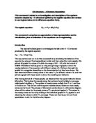
Now that we have observed the logistic equation responding to different values of k, we were set the task of plotting the steady value of PN against the value of k. This was done simply by setting up a graph on Excel with k as the X axis and by plotting one of the steady state values against it. For the values of k which had more than one steady value we plotted these again on top of the original graph to build up a complete understanding of what happens in a bifurcation diagram.
Figure 24
This bifurcation diagram shows how the behaviour of the logistic equation can suddenly change at certain points. After doing research on the logistic equation we noticed that a strong relation to the logistic equation is the bifurcation diagram. A more detailed example of this can be seen below in Figure 45 [1]. In Figure we can see how our diagram matches the same diagram for a slightly different logistic equation. They both break onto chaos very quickly after the first bifurcation, and the distance between the following bifurcations decreases dramatically each time. In Weisstein’s diagram Figure 45[1] he has plotted after the diagram reaches chaos, therefore we went back and plotted a few more of the values that we acquired for the values of k after 2.5625 in order to see if we could see if a trend was occurring. This diagram also shows where the bifurcations occur.
Figure 45[1]
Figure 46
Figure 46 is a version of our bifurcation diagram, with sample values from the graphs which didn’t converge to any steady states. It shows how in our equation, chaos takes over very rapidly. If we had plotted more values for the chaotic values of k, we would have seen a closer relationship to the graph above it.
Finding δ and α
While looking into bifurcation how the distance between each bifurcation brought up Feigenbaum constant, a good description of this was illustrated on Wolfram Alpha[2] they described it as “The Feigenbaum constant δ is a universal constant for functions approaching chaos via period doubling” [2]. Therefore, this implies that there is a ratio that governs the distance between each bifurcation. It also suggests that this value can be used for any dynamic system as long as it shows period doubling, and due to the fact that our system does this we can apply this to our results. So there exists an equation to solve for δ.
[2]
Figure 47
When implemented this equation should give a value of 4.6692[2].
The other Feigenbaum constant α is “defined as the separation of adjacent elements of period doubled attractors from one double to the next”, just like δ it’s a ratio for the bifurcation diagram. When the diagram’s steady states multiply, it describes the distance between the values. It is calculated by:
[2]
Figure 48
This equation gives a value of 2.5029[2].
Using appropriate cited evidence from the literature, describe TWO engineering applications where the Logistic equation has been used to model or simulate real world phenomena.
Application 1- Chaotic noise MOS generator based on logistic map
Introduction: what it is simulating?
One of the engineering applications where the Logistic equation has been used to simulate real world phenomena is with an analog noise generator. This noise generator simulates the behavior of an electronic circuit which is iterated using a current amplifier with the gain μ[3], in the same way that our equation is iterated with the gain k. In this case the logistic equation is;
f(x(n)) = x(n+1) = μ x(n) (1-x(n))
It is simulating an analogue noise MOS generator circuit using different values of μ to find the steady state of the current. The logistic equation and a bifurcation diagram are used to study the behaviour of the system to help in the design of the circuit. Certain conditions are needed for the circuit to run smoothly, and to find what these specific conditions are, a logistic equation is used to study the effects of using different values for the gain in current. Different graphs are plotted of transient analysis, for different values of μ to analyse the behaviour at intervals, shown in fig 50. The steady states are then taken from these graphs to plot on the bifurcation diagram, shown in fig 51.
How the logistic equation is used
In this application the logistic equation is used in circuit design as a model to mathematically simulate the behaviour of the circuit in order to find the stable values for the current. The logistic equation works alongside Lyapunov’s experiment and Birkhoff’s Ergodic Theorem in the design of the circuit, but the model is mainly governed by the logistic equation.
In transferring the logistic equation into practical use in the analogue noise MOS generator circuit, the equation simulates an amplifier of current with a gain of μ. The differing values of μ affect the transfer function in the circuit. The bifurcation diagram and Lyapunov’s experiment work together to indentify the steady states due to the logistic equation, and this is used in the design of the circuit, as these steady states are to be avoided.
The Logistic Equation has chaotic behaviour as there is no set pattern and the numbers randomly change, which we found by plotting the graphs.
How this application relates to bifurcation
In this application the logistic map of the chaotic noise MOS generator shows chaotic behaviour.
The variable μ in this application has the same function as the variable we called k in our work, it is known as the control parameter. Values for x are taken between 0 and 1, and values for μ are taken between 0 and 4.
In the same way that our bifurcation diagram only converged to one steady state for values of k below 2, for values of μ below 3 the values for x(n+1) converge to one steady state also. Similarly, as in our work when k is increased for values above 2, when μ is increased to values over 3, there are now 2 steady states. Furthermore, as μ is increased between the values of 3 and 4, the number of steady states reached also increases from 4 to 8 and then to 16. This is reflected in our own bifurcation diagram, as the value of k is increased between 2 and 2.567. The number of steady states is increased also, in the same way.
The bifurcation diagram shows the system behaviour; where one steady state turns to two steady states, the line is shown to split into two on the diagram, as shown in fig 51[3]. Likewise, 4 steady states emerge, then 8 and then 16 steady states the lines are shown to split further until the system develops into chaos.
In this system, as μ reaches values greater than 3.5699456[3], there are no longer any steady states reached. The values for x(n) never converge and reach steady states. This is because the system is now in chaos, which is shown on the diagram as the shaded region. This relates to our work as the logistic equation we used reaches chaos, at which point the value of k is 2.567.
Application 2- Image encryption using chaotic logistic map
Introduction
Through the course of time, the world has advanced through many ages, be it the middle ages or the ongoing digital age. With each age humanity has made great strives at improving themselves and their environment, various innovative ideas have been put forward and developed but as the case is with most, with each new innovation comes a whole new set of barriers.
“Encryption is the conversion of data into a form, called a cipher text, that cannot be easily understood by unauthorized people (searchsecurity.com © 2000 contributors Robert Bauchle, Fred Hazen, John Lund, Gabe Oakley, and Frank Rundatz)”. In recent years, with the advancement of technology, the world has become a global village where information can be sent half way across the world in a matter of seconds as a result the demand/flow of information in the form of data has risen exponentially and being able to secure your flow of data has become a necessity, it is this desideratum that brought about encryption and its uses/ methods.
Take the military for example, in war time situations communication is ‘sine que non’ for the military, not only do they need to be able to communicate with each other, they also need to be able stop the enemy from intercepting their communications. Apart from its military uses, encryption is also essential in private video conferencing, cable TV, storing personal data online and many other applications.
The high demand for encryption has lead to numerous advancements in encryption techniques as well as their algorithms, one of them being chaos based encryption techniques. Chaos based encryption techniques are praised for their good practical use, this is because of the high speed, complexity security and more they provide, an example of this can be seen in the Image encryption using chaotic logistic map article by N.K. Pareek, Vinod Patidar, K.K. Sud:-
“Digital images have certain characteristics such as: redundancy of data, strong correlation among adjacent pixels, being less sensitive as compared to the text data i.e. a tiny change in the attribute of any pixel of the image does not drastically degrade the quality of the image and bulk capacity of data etc. (© Image encryption using chaotic logistic map article by N.K. Pareek, Vinod Patidar, K.K. Sud)”.
Various methods of chaos based encryption techniques, each with their own pro’s and con’s ranging from its intended use. For real time image encryption, ciphers which take less time and yet still provide the necessary security are preferred to those which take considerably long amounts of time and produce high levels of security, this is because the latter would bee of little use in real time proceses and applications as well as the fact that as the strength of the encryption rises so does its cost.
In the case of real time imaging, chaos based encryption have been seen as a best fit, various chaos based image encryption schemes have been developed, each one aimed at being able to provide a quick ad yet still highly secured means of image encryption, with a novel image encryption scheme based on the logistic map and cheat image being an example.
How is the logistic equation used?
In image encryption a process called decryption is used using logistic maps. Chaos is a spectacle that occurs in nonlinear systems which are highly sensitive to initial values. These tend to show random behaviour. If a system is in chaotic mode it has to satisfy the condition of the equation.
Any minor variation of the initial values can cause considerable differences in the next value of the function, that is, when the initial signals varies a little, the resulting signal will change significantly.
Methods such as random number generators are used in chaotic function algorithms as they are able to regenerate the same random numbers, having the initial value and the transformed function.
Xn+1 = rXn (1-Xn)
This equation is one of the most knows equation to display random behaviour, it is known as a logistic map signal. Throughout the algorithm, we keep the value of the system parameter of the both logistic maps to be constant which can be described as a highly chaotic state.
This signal will have chaotic behaviour in case the initial value X0 e (0,1) and r=3.999 which is a constant. If you look at figure 2 the signal behaviour with initial value is X0 = 0.5 and r =3.999 can be seen.
References
[1] Weisstein and Eric W: "Logistic Map", From --A Wolfram Web Resource, http://mathworld.wolfram.com/LogisticMap.html, accessed November 18th 2011.
[2] Weisstein and Eric W: "Feigenbaum Constant", From --A Wolfram Web Resource, http://mathworld.wolfram.com/FeigenbaumConstant.html, accessed November 18th 2011.
[3] A. Díaz-Méndez, J.V. Marquina-Pérez, M. Cruz-Irisson, R. Vázquez-Medina, J.L. Del-Río-Correa: “Chaotic noise MOS generator based on logistic map”, Microelectronics Journal, Volume 40, March 2009 [accessed November 18th 2011], available from: http://www.sciencedirect.com/science?_ob=MiamiImageURL&_cid=271437&_user=122878&_pii=S0026269208003091&_check=y&_origin=&_coverDate=31-Mar-2009&view=c&wchp=dGLbVlV-zSkzS&md5=2955dab1b0aa1036f7843dad878d8955/1-s2.0-S0026269208003091-main.pdf
[4] R. Vázquez-Medina, A. Díaz-Méndez, J.L. del Río-Correa, J. López-Hernández: “Design of chaotic analog noise generators with logistic map
and MOS QT circuits”, Chaos, Solitons & Fractals, Volume 40, 30 May 2009 [accessed November 18th 2011], available from: http://www.sciencedirect.com/science?_ob=MiamiImageURL&_cid=271591&_user=122878&_pii=S0960077907008089&_check=y&_origin=&_coverDate=30-May-2009&view=c&wchp=dGLbVlk-zSkzS&md5=6ac3c93797f9ff3a26f5c7062f58f36e/1-s2.0-S0960077907008089-main.pdf
[5] N.K. Pareek, Vinod Patidar, K.K. Sud: “Image encryption using chaotic logistic map”, Image and Vision Computing, Volume 24, 1 September 2006 [accessed November 18th 2011], Pages 926-934, available from: http://www.sciencedirect.com/science?_ob=MiamiImageURL&_cid=271526&_user=122878&_pii=S026288560600103X&_check=y&_origin=search&_coverDate=01-Sep-2006&view=c&wchp=dGLzVlS-zSkWA&md5=f26352af24c8645f4778ad9458956452/1-s2.0-S026288560600103X-main.pdf
[6] Bauchle, Robert, Fred Hazen, John Lund, Gabe Oakley, Frank Rundatz: "What Is Encryption? - Definition from Whatis.com.", July 2000, accessed 04 Dec. 2011, available from: http://searchsecurity.techtarget.com/definition/encryption.