Data Analysis and Time Series Graph
The data below displays the total turnover (in million euros) of ‘Orange’ group on a quarterly basis for the period 2000 to 2003.
Quarterly Sales Turnover
Table 1.1
A close look at the data will show that the sales in Q1 start off at a low level and show a marginal increasing trend in Q2, Q3 and Q4 except in Q2 of 2002 and Q4 of 2003 where it declines compared to the previous quarter. Thus the overall turnover is low in the first quarter of every year and increases over the rest of the year. Orange provides various discounted offers and monthly contract schemes particularly during Christmas to attract more customers to use the network which increases revenue mainly during the last quarter of every year.
Following is the graphical representation of the above data:
The graph displays an increasing trend in the turnover for Orange group over the 4 years. The scrutiny of the graph enables us to identify a pattern and an approach to the analysis.
One of the traditional methods employed for modelling time series is known as the ‘decomposition approach’ which is based on the proposition that empirical evidence suggests that most series consist of:
- Long term secular trend
- Cyclical variation
- Seasonal variation
- Residual error
Noticing a peculiar cycle or pattern in the above graph, a suggested approach here would be the method of moving averages; a successive averaging process where the order of the moving average is the number of data points averaged each time. This process is sometimes known as ‘smoothing’ and the choice of order of the moving average must be made so as to best smooth out the regular variations in the data. The moving average contains a ‘lag’ effect as it reflects the values of past data; this may be corrected by calculating the centred moving average.
After observing the trends in the above graphed data, we need to isolate the seasonal component. We shall also evaluate the two approaches used to forecast i.e. the additive model and the multiplicative model of time series to decide which approach would provide a more reliable forecast. The following calculations in the table below (Table 2.1) and the approach followed will explain the process in a more systematic manner.
Calculations and Approach
Table 2.1
The actual trend (excluding forecast) calculated in table 2.1 has now been plotted in the graph below where we can notice the rapidly rising trend values.
Approach Followed:
The following steps have been followed to arrive at the calculations in table 2.1:
Step 1:
List all the actual sales figures in million euros for the respective quarter from 2000 to 2003.
Step 2:
Calculate the ‘moving annual total’ for every quarter based on the sales figures.
Step 3:
Calculate the 4th order ‘moving average’ of the totals found in step 2.
Step 4:
Calculate the Centred Moving Average (TREND) based on the moving average in step 3. The middle of the year falls between Q2 and Q3 and the original data relates to specific quarter. So to solve this problem, centred moving averages are used.
Step 5:
Calculate the ‘Seasonal Effect’ which is the difference between the actual sales and the Centred Moving average (trend) of the respective quarters.
Step 6:
Calculate the seasonal variation or the ‘Mean Seasonal Effect’ (MSE) as shown in table 2.2 below.
Table 2.2
Step 7:
Based on the adjusted seasonal variation, a final forecast was made for quarter 1 of 2004.
However we need to decide whether to use the Additive or the Multiplicative model to calculate the forecast.
Additive Model:
As seen in table 2.2 above, the seasonal effect for each quarter has the same sign in that quarter from 2000 to 2003. Also in Q3 the positive effect is constantly increasing which is very optimistic. However we also notice that in Q1, the pattern of decline is not constant i.e. it moves from -121 to – 28.75 and then again declines to – 184. Similarly in Q2 the negative effect is not constant and in Q4 the positive effect moves down from 178.38 to 119.75 and then up again to 176.75. However after referring to these historical sales patterns, I have noticed that there is no particular evidence of any specific events or occurrences at Orange for this inconsistent pattern. Since the same sign and effect exists through the quarter, the additive model is a more reliable and an appropriate approach to forecast the sales for Orange (2004, Q1).
Multiplicative Model:
However we shall also look at the multiplicative model to see if it could be a better measure of forecast. Table 2.3 below shows the calculations of the multiplicative model for the respective quarters.
Here we calculate the Actual revenue as a percentage of the Trend. Thus we have:
Actual Sales x 100
Trend
Table 2.3
For the multiplicative model to be reliable, the actual sales as a percentage of the trend for the particular quarter should be same or approximately very close. After replacing the figures in the above formula we see that the Multiplicative Model gives us big differences in the percentages in the same quarter for the four years. For example in 2001 Q2, we get an effect of 99.34% compared to 94.89 % in 2002 Q2, which is not very close. With these major differences, the multiplicative model would not provide a very reliable forecast and therefore it is advisable to use the Additive Model of time series.
In table 2.2 (Mean Seasonal Effect) we note that the seasonal effect is different for the same quarter in the four years. This is due to the random element. Thus the Mean Seasonal Effect (MSE) shown in table 2.2 is not a perfect result and has a total error of 18.08. So we need to correct this error by smoothening out the seasonal variations to arrive at values without errors using the additive model of time series. We therefore divide the error (18.08) equally amongst the four quarters to arrive at an adjusted MSE. This will enable us to calculate a more accurate forecast for quarter 1 of 2004.
We then calculate the Residual Error, as shown in table 2.1, in the following way:
Using the additive model of time series we get:
Y = T + C +S + E where:
Y = Actual sales
T = Long term, secular, trend
C = Cyclical variation
S = Seasonal variation
E = Residual error
After calculating the trend and the seasonal effect, we substitute the information in the formula (Y = T + C + S + E) to get the Residual errors. Here the Cyclical variation is zero.
Forecasting
Our purpose of the time series analysis above is to use the results to forecast future values of the series using the decomposition model. The procedure for this is to extrapolate the trend into the future and then apply the seasonal component to the forecast trend.
To calculate the forecasted sales for Orange group for Q1 of 2004 we take the difference between the last trend (2003) and the first trend (2000) as shown in table 2.1 (4476.5 - 3119.38) which is1357.13. This difference is then divided by 11 (no. of changes between the quarters) to give us 123.38. This is the difference on an average between the quarterly trends. which is then added to the last trend figure (4476.5) to give us the next trend figure of 4599.88 (4476.5 + 123.38).
Now to calculate the forecast we need to go backwards:
Let the forecasted revenue for Q1 of 2004 be ‘x’:
So to find the value of ‘x’:
4,255 + 4,360 + 4,714 + 4,612
+ 4,360 + 4,714 + 4,612 + ‘x’ = 4599.88
8
Thus the value of ‘x’ = 5172.
Thus the forecasted sales revenue for Orange in quarter 1 of 2004 is 5172 million euros with the forecasted trend being 4599.88 million euros as shown in the graph above.
We have now evaluated and analysed the sales data for Orange over 16 quarters from 2000 to 2003. By suggesting an approach to the analysis we have also projected the forecast for quarter 1 of 2004 and we shall now move on to comparison.
After calculating the forecast I compared the forecasted figure to the actual sales for the first quarter of 2004 which was given as 5000 million euros as shown in the graph above. As we can see, this is relatively optimistic and close to our calculations. The reason for the forecast being close to the actual sales, I believe, is the use of additive model of moving averages, which smoothens the data leaving no room for seasonal errors thus arriving at a seasonally adjusted forecast for quarter 1 of 2004. Referring to the actual sales in Q1 of 2004 I noticed that the merger with France Telecom significantly improved the group’s profitability and operating margins. Solid resilience of Fixed Line, Distribution, Networks, Large Customers and Carriers segment also enabled an increase in the consolidated revenues of Orange.
Methods of forecasting based on an analysis of historical data can only provide a valid basis for predicting the future to the extent that the factors remain unchanged and the same general trends are followed in the future. There are changes and seasonal errors in the trend, which could arise due to external factors that are not taken into consideration i.e. market demand, consumer preferences, competition or changes in legislation etc.
However in calculating and evaluating the forecasted sales revenue for Orange, we have taken into account the nature of residual errors which gives us a more accurate result. Also short term forecasts are more reliable than long term forecasts as seen in our comparison of Actual v/s Forecast for quarter 1 of 2004. Thus the above approach takes into consideration seasonal errors, those we cannot control and also distributes the same between all quarters to arrive at an adjusted seasonal variation allowing an error free and a more precise forecast. We can therefore conclude that forecasting is a method by which a business can evaluate its performance which is used as s decision support process and is almost never the actual outcome but provides an idea as to what is expected under normal course of actions.
Bibliography
Morris, C. (1983) Quantitative Approaches in Business Studies 4th edition, Great Britain: Pitman Publishing.
Oakshott, Les. (1998) Essential Quantitative Methods for Business Management and Finance 2nd edition, New York: Palgrave Publishers Ltd.
Friend, D.V. (1987) Quantitative Methods (Longman exam guides) 2nd edition, United States of America: Longman Inc.,
Information and sales revenue data of the Orange group (2004), Available:
Last accessed: 18th November 2004
Word Count: 1420 words
Figures in blue contribute towards forecasted sales for 2004, quarter 1.