How does this influence the behavior of the electrons? We get the answer by regarding electrons as waves passing the crystal. Bragg reflection occurs for wavelengths in the range of the lattice constant. The diffraction condition in reciprocal space is given as
Where is the wave vector with direction of wave propagation and magnitude. The one dimensional equation reduces to
with as the one dimensional reciprocal lattice vector. Equation 2.1.3 gives us the borders of all the Brillouin zones. No wave Ψ = A exp(ikx) with wave vector matching 2.1.3 can pass undisturbed through the sample. Diffraction will cause an equal distribution of waves in both directions. The result is a standing wave. Let us have a look at waves with wave vector k = 2π/a (n = 1). There are two possible standing wave solutions, the time independent amplitudes can be written as
Let us have a look where these two solutions concentrate the electron charge density. The distribution of charge density ρ = Φ∗Φ is given by the following equations:
Solution Φ− concentrates the charge density between the atoms where the periodic potential approaches a minimum. Solution Φ+ results in charge concentration near the cores where the periodic potential is highest. The reason for the band gap in periodic structures is to be found in this difference in potential energy of the two wave solutions. Calculations in three dimensions follow the same approach. The derivation of the band gap in real lattices is a complicated task that can just be solved by numerical calculations.
In this experiment, the wavelength dependent optical absorption for semiconductor samples; Gallium Phosphate (GaP) and Gallium Arsenide (GaAs), were measured.
The experimental assembly provides electromagnetic radiation in the wide range of 380nm to 1080nm. This range makes several interaction processes with matter possible. In the long wavelength limit radiation can excite free charge carriers to oscillate causing reflection. In short wavelength limit radiation has enough energy to interact with inner shell electrons. The typical band gap energy of semiconductors is found in between these extremes. Light cannot be absorbed when electrons would acquire the amount of energy to find themselves in the forbidden zone between the bands. Just photons with energy high enough manage to catapult electrons over the gap. We should therefore find a strong increase of absorption probability when the energy of a photon exceeds the energy of the band gap. This is displayed as changes in output signal intensity. The bandgap energy of each semiconductor crystal can be found using the following equation:
Where plancks constant, speed of light in a vacuum and the wavelength where the absorption becomes non-zero. By plotting the transmission constant (the ratio of , where is the intensity reading without a sample) against the corresponding wavelength, the x-axis intercept of the from the absorption edge region gives .
Semiconductors can be classified into two types, namely direct gap and indirect gap
materials. GaAs is a direct gap semiconductor. The absorption spectrum for a direct gap material is shown in Figure 2(a). Note that there is a very sharp absorption edge that starts at an energy equal to. For an indirect semiconductor such as GaP, the energy gap is more complicated, resulting in a secondary absorption edge, as shown in Figure 2(b). Indirect gap semiconductors include Si and Ge
Figure 2.2
Optical absorption in pure insulators at absolute zero.
- Experimental Method
A Source of variable wavelength, monochromatic, light is obtained using a 100 W Quartz-Halogen (QTH) bulb in a housing that allows the light to be focused on the entrance slit of a grating monochromator. The lamp is powered by a FARNELL B30/10 power supply. This monochromator uses a diffraction grating in order to allow the wavelength of light that is brought to focus at the exit slit can be analyzed by rotating the grating.
Figure 3.1
Grating monochromator showing how the initial beam of white
light is split up using the rotating grating
The light emerging from the monochromator is detected by a Si-Based photodetector, between the monochromator and the detector. The intensities of the detected signals are very small and can be comparable to the noise amplitude so a lock-in amplifier in combination with an optical chopper was used to allow detection. The chopper modulates the light intensity passing through the monochromator, and the phase sensitive detector circuitry only amplifies signals with a narrow bandwidth about the modulating frequency. Stray light, not passing through the chopper will not give a detectable signal from the lock-in amplifier.
The power supply was turned to the 0-6V scale and the fine control was set to minimum before it was switched on. The power supply was then switched and set to the
6-12V range, allowing several minutes to heat up. The voltage was then increased by increasing the fine control, rotating it to approximately 75% full scale. The light was focused on the entrance slit of the monochromator, through the chopper blades.
The chopper was then switched on and set to a frequency of 410Hz.The lock-in amplifier and DC voltmeter was then switched on and set to the following criteria: Sensitivity to 100mv, input A was used. The filter was set to BP (Bandpass) and MAN, and the line reject filter was set to F. The tuning display will show the chopper frequency. The output time constant was set to 300ms with a slope of 6dB and the output mode NORM.
The wavelength on the monochromator was then switched to 1080nm and readings were taken (using no sample) every 20nm from 1080nm to 380nm and the response plotted. The photodetector housing was removed and the GaAs sample was mounted over it. Readings were then taken over the same range, again every 20nm. The GaAs sample was then replaced by the GaP sample and the experiment was carried out again. The Transmission constants were then plotted against wavelength as previously stated in the introduction. From these plots, the approximate positions for the absorption edges were indentified and more detailed measurements were carried out over these regions. These graphs were used in collaboration with to find the bandgap energies of each of the two semiconductors.
- Results and Discussion
A full set of measurements were taken for both semiconductors over the given range however when these results were plotted, the formed graphs did not follow the suspected relationship. This was due to the output frequency gradually going out of phase when the wavelength and samples were changed causing massive errors. There results were then ignored and the experiment was re-started.
Readings were then taken for both samples and the response frequency(no sample) over the range previously stated(1080nm to 380nm) making sure the output signal was always in phase, using the lock-in amplifier, every time the wavelength was altered. The tables of these results can be found in Figure 7.1 of the appendix.
The results were then plotted in order to indentify the position of the absorption edges.
Figure 4.1
Graph of GaAs Transmission constant against wavelength
Figure 4.2
Graph of GaP Transmission constant against wavelength
From these graphs it was clear that the absorption edges for GaAs and GaP were between wavelengths (800-1000)nm and (500-650)nm respectively. The absorptions edges were then analyzed by taking readings over these wavelength regions in smaller increments for the corresponding semiconductors. Tables of these results may be found in figure 7.2 and figure 7.3 in the appendix. The following graph for the absorption edge of GaAs was obtained.( Graph of GaP can be found in figure 7.4 the appendix)
Figure 4.3
Graph of GaAs absorption edge
Using the linest function in excel, the gradient and intercept were found to be;
Figure 4.4
Linest table for GaAs Absorption edge
Were the intercept represents. Therefore by using the value of the bandgap energy for GaAs was found to be 1.404eV. This process was repeated for the GaP sample and its corresponding bandgap was found to be 2.33eV.
The experiment was repeated to clarify our readings and try and reduce our errors. A table of these results and bandgap plots can be found in the appendix.
From these sets of results, the bandgaps for GaAs and GaP were found to be 1.409eV and 2.34eV respectively. By using the law of averages, we can combine our two results to form:
Figure 4.5
Table of Finalised Bandgap Energies
These values coincide with published values for GaAs and GaP at 300k of 1.43eV and 2.26eV respectively
- Conclusion
We conclude that transmission spectra of a given semiconducting sample are just sufficient to calculate its energy band gap value. We have verified this method for two semiconducting materials, GaAs and GaP and found this an accurate and fastest for energy band gap determination. Measurements of the transmission constants of both the GaAs and the GaP semiconductor samples gave, using the accepted value for the speed of light and Planck’s constant, energy values of (1.41 and 2.33)eV respectively which are consistent with accepted values of (1.43 and 2.26)eV for the bandgap energies measured at 300K.
- References
[1] O.S. Heavens, Optical Properties of Thin Solid Films, Butterworth, London, 1955.
[2] F. Tepehan, N. Ozer, Solar Energy Materials and Solar Cells 30 (1993) 353.
[3] T.P. Sharma, S.K. Sharma, V. Singh, C.S.I.O. Communication 19 (3±4) (1992) 63.
[4] V. Kumar, V. Singh, S.K. Sharma, T.P. Sharma, Optical Materials 11 (1998) 29.
[5] V. Kumar, T.P. Sharma, Optical Materials 10 (1998) 253.
[6] S.K. Sharma, V. Kumar, S. Sirohi, S.K. Kaushish, T.P.Sharma, C.S.I.O. Communications 4 (3) (1996) 189.
[7] J. Tauc (Ed.), Amorphous and Liquid Semiconductor, Plenum Press, New York, 1974, p. 159.
- Appendix
Figure 7.1
Table of results showing the intensities of the output signal and transmission constants
Figure 7.2
Table of results showing the transmission constants for the absorption edge analysis of GaAs
Figure 7.3
Table of results showing the transmission constants for the absorption edge analysis of GaP
Figure 7.4
Graph of GaP Absorption Edge for Run 1
Figure 7.5
Graph of GaP Absorption Edge for Run 2
Figure 7.6
Graph of GaAs Absorption Edge for Run 2
Figure 7.7
Table of Transmission Constants of GaAs Absorption Edge for Run 2
Figure 7.8
Table of Transmission Constants of GaP Absorption Edge for Run 2