The aim of this experiment was to set up, calibrate and use a model focimeter to measure the power of an unknown lens.
The Vertex Focimeter.
Aim:
The aim of this experiment was to set up, calibrate and use a model focimeter to measure the power of an unknown lens.
Introduction:
Carl Zeiss developed the focimeter in order to measure the power of an unknown lens, however it was C.J. Troppman who produced the model that we use now. The power of a lens is said to be the ability of the surface to alter the curvature of light, i.e. altering the vergence of the incident light.
The need for the focimeter in optical practices is that it enables us to identify the patients prescription from their spectacles, which in turn allows technicians to check whether the final spectacles are of the write prescription. The focimeter can also be modified slightly to measure the vertex power of hard and soft contact lenses. There are several methods of determining the back vertex power of a lens, some of which are more accurate than others.
* Neutralisation:- By superimposing trial case lenses of known power on the unknown lens a combination can be found whereby there will be no movement of the image of the target. At this point the unknown lens has been neutralised and its power is equivalent to that of the trial case lenses but with opposite sign. In order to ensure accuracy the neutralising lens must be placed in contact with the back surface of the spectacle lens. This is not always possible with some curved lenses leaving a 3-6mm gap which more often than not affects the accuracy of the result. Therefore it has become very common for trial lenses to be placed against the front surface of spectacle lenses whereby the front focal power is measured. The front vertex power is not the same as the back vertex power (which in most cases is stronger) and therefore this technique is not accurate enough when lenses have powers of more than two dioptres.
* Lens Measure:- Geneva Lens measures can be used to find the powers of a lens measuring the surface curvature. The total power of a thin lens equals the sum of its surface powers, however it cannot be assumed that ever unknown lens is thin. Furthermore the instrument is calibrated specifically for crown glass (refractive index =1.523) and is therefore unsuitable for determining powers of a lens of another material (different refractive index).
* Eyepiece Focimeter:- Originating in 1910, the conventional design makes it a user-friendly tool in determining the power of an unknown lens. The optical system depends on the skill of the operator in correctly adjusting the position of the eyepiece using manual controls and judging the position of best focus. A focimeter can also be used to check the cylindrical lens power and axis, as well as the prismatic correction (both power and direction) and the optical centres of the lens.
* Projection Focimeter:- A projection focimeter works in a similar fashion to the eyepiece focimeter, i.e. the lens to be measured is introduced into the optical beam path of the system, thus throwing the system out of focus, and the system is then refocused. Again refocusing relies on the judgement of the operator, however with a projection focimeter the image is magnified onto a screen. Once focused the power can be read off another screen. Having a magnified image projected on another screen reduces errors on the part of the examiner by making focusing more precise and preventing accommodation. Furthermore this screen can be viewed by several people who can then concur the results without having to make adjustments.
The picture below is of a Projection Focimeter:-
* The Focimeter measures back vertex power.
* Front or back vertex power depends on the orientation
* Projection focimeters avoid errors due to proximal accommodation
* The standard lens must be more powerful than the standard lens to be measured.
* Automatic Focimeter:- This works in a similar way to the other focimeters, however the judgement of the operator is replaced by photo sensors and electronic circuitry i.e. it is automated. These focimeters can be obtained in two basic versions. The first still allows the operator to focus a target on a screen and a power is then read off from a digital screen. As an alternative, the whole operation can be fully automatic. With the second type the operator only needs to put the lens in place and adjust one or two controls which allows a less experienced operator to use this instrument. Another advantage of this machine is its ability to display the sphere and cylinder powers rather than the cross cylinder form which avoids the problem of incorrect mental arithmetic when converting to sphere/cylinder form.
For the purpose of this experiment a eyepiece focimeter was setup, it would allow us to gather more accurate results over a wider range of powers in comparison to a lens measure and hand neutralisation using trial case lenses. Both a projection focimeter and an automatic focimeter could not really be considered, as the optical systems involved in preparing them would have been far too complicated for inexperienced individuals such as us. Therefore it seemed fit that we had to compromise simplicity in model design and having to manually focus the eyepiece of the telescope.
Theory:
...
This is a preview of the whole essay
For the purpose of this experiment a eyepiece focimeter was setup, it would allow us to gather more accurate results over a wider range of powers in comparison to a lens measure and hand neutralisation using trial case lenses. Both a projection focimeter and an automatic focimeter could not really be considered, as the optical systems involved in preparing them would have been far too complicated for inexperienced individuals such as us. Therefore it seemed fit that we had to compromise simplicity in model design and having to manually focus the eyepiece of the telescope.
Theory:
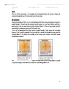
The focimeter is based on Newton's equation:
-x . x' = (f)2
Where:- x = object distance measured from the front focal point,
x' = image distance measured from the back focal point,
(f) = back focal length of the lens which is assumed to be in air.
The vertex focimeter is not the only way of measuring the power of an unknown lens, there is a technique of neutralization which involves placing lenses of known power and opposite sign in front of the unknown lens. This is done until the with or against movements of a distant image disappear at reversal. Therefore the unknown lens will have the opposite power to the lens that neutralized it. This method however takes a lot of time and is not as accurate as one cannot be certain that the power of the neutralizing lens and the power of the unknown lens are exactly the same.
Another technique involves using the Abbe Refractometer, it is used initially to find the refractive index of a lens. This is then followed by finding the radius of curvature using a Spherometer. Both techniques are accurate but consume much time and are therefore unpractical. The advantage of using the vertex focimeter is not only is it quick and simple but the fact it can measure both positive and negative lenses over wide range.
The triangle ABF' is similar to triangle O'P'F' therefore AB/O'P' = AF'/O'F'
But AB = h, O'P' = h', AF' = f', and O'F' = -x'
Hence, h/h' = f'/-x'
Triangle OPF is also similar to triangle ACF therefore OP/AC = OF/AF
But AP = h, AC = h', OF = -x, and AF = F
Hence, h/h' = -x/f
Therefore equating 1 & 2
f'/-x' = -x/f
Therefore -x.x' = f.f'
But for thin lenses in air nobject = nimage
f' = -f
and so -x . x =(f)2
Method:
Apparatus:-
* Light Source
* Collimated Telescope
* Standard Lens
* Magnifying Glass
* Variety Of Lenses (With Known and Unknown Powers)
* Positioning Stop
* Standard Lens +7.00D
* Object With Holes
* Length Of Thread
Initial Adjustments:
Using a double clamp the standard lens (+7.00D) was placed near the centre of the bench, the emphasis of the double clamp was important as movement of the lens during the experiment would affect the accuracy of the results. This was then followed by the calibration of the telescope using a standard collimator. Thus allowing the telescope to receive collimated light.
In order to do this, we looked through the eye piece of the telescope and focused on the cross wires. A plain piece of paper was then placed in front of the telescope so that a clearer image could be viewed of the cross wires. The eye piece was then inserted into the eye piece holder and the paper removed the collimator was then switched on. The draw-tube of the telescope was then pushed in and out until the cross wires could be viewed sharply. The accuracy of the calibration is vitally important because if it is done incorrectly the rest of the experiment could well be effected. To avoid any errors the telescopes eye piece, standard lens, positioning stop and the telescope objective all had to be in the same axis and at the same height. Once the calibration was done the telescope was placed between the light source and the standard lens.
The positioning stop was placed on the optical bench. In order to find the location of (F') of the standard lens the positioning stop was moved back and forth until a length of thread came into sharp focus. This adjustment was carried out five times and the giving five readings from which the mean was taken as the correct position.
When the equipment had been setup the optical centre of all the elements was aligned using a distance bar. It was particularly important to ensure that light passed through the optical centre of the test lens as when using thicker lenses the power is not the same as the periphery.
With the tungsten lamp switched on the observer looked through the telescope and the positioning stop, and located the illuminated object at the focus "F" of the lens. The mean number of readings was used for accuracy, this result being the scale point from which all movements of the objects were measured.
Then to find focal point (F) a similar procedure to locating the position stop was used. This involved viewing the target and moving it very finely both forwards and backwards until it came into fine focus. Again this was repeated five times and the mean taken as the correct position.
Using a test lens of power +1.50D with the positioning stop caused the target to come out of focus. The target was brought back into focus by moving it back towards the standard lens. This measurement was repeated three times for the +1.50D lens and the mean was taken as the correct position and recorded. This process was repeated with two more positive lenses of powers +2.00D and +3.00D and it was repeated with three negative lenses of powers -2.50D, -6.00D and -8.00D.
Results:-
Reading Number
Position Stop (mm)
13.6.9
2
137.2
3
137.3
4
136.8
5
137.5
Mean
137.1
The table above gives the five values taken to find (F') i.e. the position stop. The mean value was found to be 1137.1mm this was taken as the position stop.
Reading Number
Target Position (mm)
858.1
2
858.4
3
858.0
4
858.3
5
858.3
Mean
858.3
The table above gives the five values taken to find (F) i.e. the Target position. The mean value was found to be 858.3mm this was taken as the Target position.
The table below gives all the readings and the means for the values of the known lenses found during the experiment:-
Lens Power (D)
Position Of Object B (mm)
Mean Value for position B (mm)
S.D.
?
Distance x (mm)
+1.50
888.4
888.5
888.2
888.4
0.1528
?0.0882
28.90
+2.00
898.0
898.6
898.3
898.3
0.3000
?0.1732
38.80
+3.00
919.9
918.7
918.6
919.1
0.7234
?0.4177
59.60
-2.50
805.4
805.0
806.7
805.7
0.8888
?0.5132
-53.80
-6.00
729.9
731.4
731.1
730.8
0.7937
?0.4583
-128.70
-8.00
688.9
689.1
690.3
689.4
0.7527
?0.4372
-170.10
The table below shows the results for the unknown lenses:-
Lens Power (D)
Position Of Object B (mm)
Mean Value for position B (mm)
S.D.
?
Distance x (mm)
A
898.4
900.0
899.0
899.1
0.8083
?0.4667
39.6
B
752.9
754.0
753.4
753.4
0.5508
?0.3180
-106.1
Error Analysis:-
The mean object position for unknown lens A was 899.1 ?0.4667mm.
Using the computer program entering the value 899.1 the lens was calculated to be +2.00D.
The standard error for Lens A could be calculated as follows;
?x = V?a2 + ?b2
where ? = S.E. of the distance x
? = S.E. of F
? = S.E. of Flens A
? = V (0.4790)2 + (0.4667)2
= 0.66876744
= 0.6688mm (4 dp)
From the results x = 39.6? 0.6688mm
Using the linear relationship between x and the BVP of the unknown lens.
X = Fv'
Fs2
Where y = x m = 1 x = Fv' c = y - intercept
Fs2
The formula can be rearranged in the form
X = Y - C
M
From equation
?numerator = ?y + ?c2
where ?y = S.E. of x
?c = S.E. of y-intercept
?numerator = (0.6688) + (0.5254)
= ? 0.8505mm
The mean object position for unknown lens B was 753.4 ? 0.3180mm.
Putting the mean value into the computer allowed the program to calculate the lens power to be +2.00D.
The S.E. for the power of the lens can be calculated in the same way as lens A. Using that same method the value came out be;
-4/96 ? 0.4970D
The computer then calculated the power of the lenses by interpolating the graph, however the power can be found by using the equation.
Y = MX + C
Y = 20.94104X - 2.241372
Where Y = the distance moved by x
x = power of the lens
Theoretical calibration constant (= focal length of standard lens mm)2
1000
F = n' f' = n' = 1 = 0.142857142m
f' F F = 142.857142mm
Calibration constant = (142.857142)2
1000
= 20.40816327mm/D which also equals gradient of graph
Practical Calibration constant = 20.94104 ? 0.1261026
Normal Distribution calculation for checking whether result where due to chance or not.
For Lens A, (= 898.1mm SD = 0.8083 mm n= 6 (sample size)
We take the test statistic as the standard error + the Mean value = 899.768
Therefore we are doing a two Tailed Test with:
Ho (null hypothesis) as that the results are not significant
H1 (alternative hypothesis) that the results are significant
And are doing the test at a 5% significance Level.
Standard Deviation = 0.8083 therefore the variance of the sample = SD2= 0.65334
Therefore the population variance = n/(n-1) x Sample Variance
= 6/5 x 0.653354
= 0.7840
And the mean stays the same for the population
Therefore test statistic = 899.768
P(X>899.768) = P(X>Z)
Z = (899.768- 898.1) / 0.7840 <-- this stage converts it into a Z(0,1) Normal distribution.
Therefore Z = 2.12755102
Therefore the probability that P(X>2.12755102) = 0.0167 or 1.67%
At the Significance level 5% as it is a two tailed test, 1.67% < 2.5% therefore at the 5% significance level we can justifying say that the results I obtained where significant.
With Lens B the results are also significant with probability being 1.297 which Is less than 2.5% therefore can reject the null hypothesis at 5% level.
Discussion
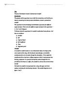
The relationship this experiment was based upon was Newton's equation from which the focimeter equation was derived. The linear relationship between x the BVP was expected to be a straight-line graph through the origin.
X = Fv' where 1 = gradient
Fs2 Fs2
However the calibration graph plotted from the results had an intercept of -2.241372 mm with a standard error of ?0.5253674 mm and a gradient of 20.94104 mm/D with S.E. of 0.1231026 mm/D.
It is easier to see the implications of these errors in the results in graphical form.
The graph has the possibility of having a gradient within the standard error of ?0.1261026 mm/D.
The practical calibration constant was worked out to be 20.94104 ?0.1261026 mm/D.
The experiment assumes that the optical centre of the lens of the telescope, positioning stop of the object are all aligned along the same axis. Checking this practically depends on human judgment. Horizontally use of the distance bar is a more accurate method than checking the alignment from above where there is a limitation due to the bench being too high. Because of this it cannot be said that the stop is centrally aligned, which means that both F and F' are slightly out of position.
There was a slight difference in the apparatus used to focus both F and F'. In the case of F' a piece of string was used whereas in the case of F the object was illuminated with light. In this case it was easier to notice when the string came into sharp focus whereas it was difficult to see the contrast in the object.
Since the experiment used lenses which had a wide range between them i.e. -8.00D - +3.00D. from the results it can be seen that both the S.D. and the S.E. generally increase in the same order that the lenses were tested. The factors that could have contributed to this trend are that one person took the measurements for consistency and in order to make the experiment fair. This however may have also led to eye strain as the experiment progressed which in turn affects the results. Another error may have been the position of the lens vertex relative to F'. As the surface becomes more curved there is greater difference in the position of F' and the vertex. This is why the error is not so significant in the weaker powered lenses.
The negative lenses have a much higher S.D. and S.E. than the positive lenses. This may be due to the fact that the object is moved further away from the telescope therefore the error in its optical alignment with the equipment becomes more apparent, the implication being wider spread of readings and therefore the a less accurate mean position. For the negative lenses the S.D. and S.E. decrease as the negative power increases, it seems the readings become more accurate. An explanation of this in terms of resolution, as the negative power increases the distance x becomes a larger value. Therefore considering the vernier scale has an accuracy of ?0.1mm, as the length x increases, the overall error in its measurements decreases.
The positive lenses S.D. and S.E. increases as the lens power increases. A possible cause for this error may have been that the distance x is a moment away from the light source therefore the object is gradually illuminated less. The implication of this being that the contrast in the object is less and therefore it is harder to focus on it and so a greater variation is obtained.
The general accuracy of the experiment may also have been affected by the quality of the standard lens. Any aberrations in this lens will affect image quality and the accuracy of the setting, the experiment is based on parallel rays entering the telescope, if the telescope is not collimated correctly then the whole experiment is likely to be inaccurate.
Further problems involved the method of attaching the lens to the stop. For a start the blue tack left marks on the lenses which were difficult to remove and the blue tack would make it difficult to place the lenses in the correct position.
The variation in the gradient and intercept has an influence over the estimated power of the unknown lens. However the unknown lens power that the computer worked out was a simple interpolation of the graph and therefore did not take into account any of these factors. For this reason and error analysis calculation was carried out to find out the S.E. of the unknown lens power. The result was ?a = 2.00 ?0.04236D, ?a = -4.96 ?0.4770D.
The negative lens has a much higher S.E. than the positive lens however they are both small i.e. less than 1. The variation of S.E. between the positive and negative lens mirrors that the calibration graph #1 therefore assume that the errors that applied to the calibration lenses apply to the unknown lenses.
Lenses are generally with lens powers of the interval ?0.25D therefore as my S.E. are less than this interval I can conclude the lens power of A lies within the value +2.00 ?0.25D and lens B lies within the value -4.96 ?0.25D.
The whole experimental system was based around the standard lens of power +7.00D and Newton's equation -x.x' = (f)2. The level of accuracy to which the back vertex power of the standard lens was calculated is fundamental to the precision of the instrument. Trial case lenses are accurate to ?0.12D which is a suitable level of accuracy for the intended purpose of hand neutralisation, however even this small variation would introduce a systematic error when used as the standard lens in a focimeter. Similarly the powers of lenses A and B were calculated using the calibration data and would be affected by the accuracy of the powers calibration lenses. It was not possible to calculate the standard error of these lenses or of the standard lens however this source should be considered as possibly having contributed to the systematic error observed in the results. Also the derivation of Newton's equation,
-x.x' = (f)2, involves using the thin lens approximation and will not give an exactly correct result for lenses that are not 'optically thin'.
Finally to improve this experiment each measurement should be repeated at least fifty times in order to give true meaning to the statistical analysis. The full experiment should be repeated by several different people whose eyes have been tested and corrected if necessary. A more detailed target such as a grid with small squares or a small graticule should be used to improve the accuracy of focusing. A wider range of calibration lenses should be used with smaller increments in power to generate more accurate values for the gradient and y-intercept of the calibration graph. Also the powers of the standard and calibration lenses should be checked with a focimeter to determine their exact values, and finally, to make the instrument more suitable for use in optometric practise, a higher powered standard lens should have been used to account for patients with strong prescriptions.
References:
. Bennett's Ophthalmic Prescription Work, Forth Edition, - Kelvin G. Wakefield (2000), Butterworth Heinemann
2. Clinical Optics, Second Edition - A R Elkington and H J Frank (1991), Blackwell Scientific Publications
3. First Year Optics Course Manual - Dr Chris Hull (2001), City University
4. Optics Second Edition - A H Tunnacliffe and J G Hirst (1997), Association Of British Dispensing Opticians
Optics Formal Report
- 1 -