(∆K/ ∆L) = - (MPL /MPK)
As previously mentioned, a profit maximising firm will always wish to minimise costs. A budget constraint will signify the fixed sum that a firm can spend on inputs. It is the financial constraint of a firm. Capital can be given a charge of r (per unit bought) and labour can be given a price, w (wage rate per hour).
Cost of Production = wL + rK
If a firm were to spend its’ total budget on capital, it could purchase C/r, and similarly, to spend all its funds on labour, C/w could be hired. The slope of the firms’ financial constraint, or isocost, will hence be -w/r, and all other points along the line show the various purchases they could make of the inputs.
Criteria:
- An isocost line will give combinations that are equally costly
- A higher isocost line is associated with a larger budget
- The slope is linear and is the negative of the ratio of input prices (-w/r)
Diagram Isocost
‘Long run choice of inputs’
Figure 1.2 isocost & long run choices
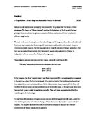
The long run labour demand curve is derived from the isocost-isoquant analysis. The point where the isocost is tangential to the isoquant is where the maximum output is achieved given the rigid budget for inputs (where MRTS = w/r). At this point, C, no higher production (or isoquant) can be reached and a lower level of output would not be optimal. This is the long run choice of labour and capital stock.
Diagram of firms optimal combination of inputs
Use 3 isoquants
Use optimal point, C
Figure 1.3 firms’ optimal combination of inputs
The long run demand curve is more elastic than the short run as the firm is able to take advantage of the economic opportunities introduced by an increase or decrease in the wage. Consider an increase in the wage to w’ and the price of capital remains at r. The isocost will readjust at the intersect C’/r but the new labour intercept will be at C’/w’. The firm will choose more units of capital and fewer hours of labour due to the augmentation of wage costs. Less hours of employment can be afforded at the higher price and the budget will take advantage of variable levels of capital instead. The slope of the new isocost has a new gradient, w’/r. Given the new market conditions, the firm will choose to be on the highest isoquant possible that the new costing slope allows. This will yield the optimal output, and will adjust the capital and labour levels accordingly. This is described as the substitution effect, as less labour, in this case, is substituted with higher levels of capital, illustrated at point B.
Alternatively, following a rise in wages, a firm might reconsider its profit maximising level of output. As it now costs more to produce goods, it could be best (i.e. more profitable) to produce less. This would be illustrated by a lower isoquant, and remaining price ratios mean that the budget line shifts inwards. This is the scale effect illustrated at point C where both inputs are inputs are proportionately cut following an increase in the cost of an output.
Diagram p.146 of LR labour demand curve
Figure 1.4 Long run labour demand curve
The downward sloping labour demand curve is determined by mapping the quantity of labour and corresponding wage costs associated with a change in the price of labour. The long run demand curve for labour therefore slopes downwards owing to both the substitution and scale effects.
b) Discuss the factors that affect the elasticity of the long run demand curve. (30%)
The concept of elasticity is diagrammatically shown by a movement along the labour demand curve. It measures the sensitivity of the quantity of labour demanded to changes in the wage rate.
The long run demand has several factors which determine its elasticity. The key features were developed by 19th century economist, Alfred Marshall in Principles of Economics.
1. Elasticity of product demand
As labour demand is derived demand, the elasticity of product demand affects the labour demand elasticity. The more elastic product demand is, the greater the elasticity of labour demand will be, cetiris paribus. This can be explained by a fall in the wage rate. If this were to occur, the cost of producing a product declines and so too does the price of the product which in turn stimulates an increase in the quantity demanded. If elasticity of product demand is great, the increase in demand for the product will increase by so much that it would be necessary to increase the quantity of labour demanded to enable the surge in production. This would indicate elastic demand for labour. An inelastic product demand would mean that the increase in product demand would be relatively low as would further labour demand. The downward sloping demand curve represents a less than perfectly elastic product demand.
FIGURE 2.1
Less than perfect product demand- price will fall as output increases
2. Ratio of labour costs to total costs
The larger the share of labour costs in total costs, the greater the elasticity of demand for labour will be. The justification of this relative importance of labour as a determinant of labour demand elasticity is explained by considering two proportions of labour costs. In the first instance, labour costs are 100 per cent of total costs and secondly, only 30 % of total costs. A 20% increase in the 100% labour costs would increase unit costs by a 20%. This increase would cause a sizeable increase in product price and therefore a decline in product sales. Eventually a large negative effect on labour demand would be seen. In the latter scenario, when labour costs are 30% of total costs, the same 20% increase would invoke only a 6% unit costs increase. This rise would result in a relatively small increase in the product price and subsequently small decline in sales and employment. The first scenario denotes a more elastic demand for labour as the same 20% increase caused a larger decline in labour demanded by firms.
3. Substitutability of other inputs
The greater the elasticity of substitution of other inputs for labour (i.e. capital), the greater the elasticity of demand for labour. If it is possible for capital to be easily substituted into labour (especially if technology has advanced capital to manage human capabilities), then a small increase in the price of labour will cause a considerable increase in the amount of machinery used in its place. A fall in the wage could result in a large replacement of labour for the relatively costly capital- if labour is substitutable (i.e. as productive or quick as the machinery for example). This illustrates elastic labour demand due to this substitutability. If capital and labour were not at all interchangeable, labour can not be substituted for capital and vice versa, and labour demand would be inelastic.
4. Supply elasticity of other inputs
Supply elasticity of other inputs elaborates of the elasticity of substitution. The greater the elasticity of supply of other inputs the demand for labour elasticity is positively affected. Elastic supply of the other inputs will meant that a small increase in the price of the input will occur in response to any given change in demand. If the supply of other factors does not expand, it would not be possible to make a substitution and demand would be inelastic.
Flat/ steep upward sloping supply curve
Change in price
as demand increases, price goes up . Therefore supply will also be affected leading to substitutability differences
FIGURE 2.1
Supply Elasticity of other inputs
c) Summarise the main findings from the empirical literature of labour demand elasticities.
(30%)
Labour demand elasticities have been vastly studied. The effect on the economy as a whole have been researched, and even more precise estimates on particular sections of the economy, such as wage elasticity of different workers from various industrial sectors, and from different countries give different elasticity measures. However, economists do agree that the labour demand curve is downward sloping and therefore elasticity is generally negative and the in the long run, labour demand is more elastic due to fewer constraints and the ability to vary capital inputs. The elasticity is still of varying degrees.
A study by Symons and Layard (1984) found elasticities for different countries were quite diverse. In their studies using Ordinary Least Squares method (OLS) of estimating elasticity, it was found that Germany, France, Japan, Canada, and Britain all had negative elasticities but USA alone has positive wage demand elasticity. Only Canada and Britain had elasticities greater than 1 indicating an elastic labour force with respect to changes in wage. The remaining nation’s elasticities were between -0.2 and -0.5, showing inelasticity and little flexibility on labour demanded irrespective of the wage set. A reduction in the wage would lead to a similar change in the total wage bill and therefore labour demanded would increase proportionately according to the magnitude of the elasticity. The disparity between countries could be accredited to the difference in measurement of output prices or due to different economic circumstances and so results are often incompatible
Table 3.1
Labour Demand Functions in Manufacturing (OLS) 1956-1980
Conversely, Bruno and Sachs (1982) found that UK elasticity for real wage in manufacturing to have an elasticity of 0.3 - much smaller than Symons and Layard’s findings. The results might be so different from the table above due to the OLS method of estimating where simultaneity bias would increase real wages after a positive shock to labour demand. A more general study on Britain’s labour demand function for the economy as a whole (i.e. all sectors) by Andrews and Nickell (1982) emerged with negative wage effects and a typically negative real wage elasticity of about -0.5.
Hamenmesh (1976) found that short term (quantified as being one year) manufacturing elasticity of labour demand in the US to be 0.32, keeping the elasticity inelastic end less so than the long(er) term estimates already discussed. For every 10 per cent change in the wage, labour demand would change in the opposite direction by 3.2 percent.
It has also been researched that the elasticity for labour demand is higher for teenagers than for adults, and also for production workers than service-sector workers. This might follow that it is higher for low skill-level workers than for high skilled/ academically demanding roles.
The significance of the findings that I have summarised on elasticity of labour demand is that public and private policies would be affected according to the change in wage rate due to the trade-off between wage and employment. Elasticity will affect the results of this trade-off. For example, if government implements a rise in the minimum wage, and the elasticity is for labour demand being inelastic (approximately 0.3 as I have summarised), a one percent rise in the wage leads to a 30 per cent drop in employment levels. Private strategies are also affected, as a union’s bargaining strategy will be influenced by the elasticity. The more inelastic the employers demand for labour, the stronger the negotiations will be to oppose a wage cut. Unions would be more uncompromising when offered a lower wage.
word count: 2098
References:
Books
Borjas, G. J. (2004), Labour Economics, 3rd Edition, McGraw-Hill
Hamermesh, D., Rees, A. (1988), The Economics of Work and Pay, 4th Edition, Harper & Row
McConnel, C. R., Brue, S. L., (1989), Contemporary Labour Economics, 2nd Edition, McGraw-Hill Book Company
Websites
Journals
Chiswick, C. U. (1985), “The Elasticity of Substitution Revsited: The effects of secular changes in labour force structure”, Journal of Labour Economics, Vol 3 No. 4, pp 490-507
Oi, W. (1962), “Labour as a quasi-fixed factor”, Journal of Political Economy, Vol 70, pp 538-55
Symons, J. and Layard, R. (1984), “Neoclassical demand for labour functions for six major economies”, Economic Journal, Vol 94, pp 788-99