-
Sheets 3 and 6 (Profit & Losses) – Whether or not a certain product was a profit or loss, the amount of profit or loss, the total money made for the week, whether or not an over all profit or loss was made from the week, the total money made or lost from all weeks, and for the 6th sheet (week 2) the average money made or lost per week.
Putting the tuck shop data and plan into a spreadsheet package (Excel):
First of all I opened up a spreadsheet packages, in this case it was, ‘Microsoft Excel’.
I inserted 6 work sheets by right clicking on a sheet tab and clicking on ‘insert…’ I then selected work sheet and clicked ok, I carried on doing this until I had 10 worksheets.
I then right clicked on each sheet tab and selected ‘Rename’. I renamed each tab with the following names:
- ‘Product Information (week 1)’
- ‘Product Expenses (week 1)’
- ‘Profit & Losses (week 1)’
- ‘Product Information (week 2)’
- ‘Product Expenses (week 2)’
- ‘Profit & Losses (week 2)’
- ‘Profit & Loss Graph (Week 1)’
- ‘Total of Products Sold (Week 1)’
- ‘Profit and Loss Graph (Week 2)’
- ‘Total of Products Sold (Week 2)’.
I entered the column headings shown above. I also labelled the sheet ‘TUCK SHOP’ and typed in the week and date, but first I had to format the cell by right clicking on it and selecting ‘Format cells’. I also wrote ‘Week 1’ to indicate which week it is.
Formatting cells
Afterwards I entered the data for ‘Quantity Bought’ which I collected from Mrs Smith.
I then entered a formula for ‘Quantity Owned’, but because this sheet was for the first week, no products were stored from the week before. So the quantity owned is the same as the quantity bought, so I entered the formula: =B5. This makes the cell equal to B5.
I then copied this formula down the column to C27 (then last product).
Formula for quantity stored
The ‘Quantity Lost’ column could not be filled in because it is the first week and therefore no products can be lost. To make this clear to the user I inserted a comment. To do this you have to right-click the cell and select ‘Insert Comment’.
You can then type in the comment and click outside the yellow box.
A red triangle will appear in the top right hand corner of the cell. When you move you mouse over it, it will appear.
The comment said, ‘Because this is the first week no products could be lost’. This is the reason why I inserted a dash because there are no products lost.
I inserted two other comments, one for quantity stored and one for quantity lost. The quantity stored comment says, ‘Because this is the first week no products could be lost’. The quantity lost says, ‘Products that can not be sold because they have been stored for over one week’.
I changed the background of cells to a light grey colour; each row was coloured grey then white e.t.c. I did this so that it is easier for a user to read the data across the sheet.
To this I had to highlight the cells I wanted to change, and then click on the background colour icon and change the colour to grey.
Changing the background colour
I froze some panes so that when you scroll down the sheet the user can still read the column names. To do this I highlighted some of the row below the area that I wanted to freeze. (In my case it was row 5) I then clicked on ‘Window’ on the taskbar and selected ‘Freeze panes’.
Freezing Panes
I changed the column widths so that the data is visible. To do this I double clicked the line between the columns and the widths automatically changed to the proper size.
I finally used the ‘Merge and Centre’ button to merge cells together where I wrote the title ‘TUCK SHOP’.
Merging cells together
I have now finished sheet 1
Sheet 3 (product information) is exactly the same apart from the data and formulas being different. The ‘Quantity Lost’ column is also different because it is the second week.
To enter the data for ‘Quantity bought’ I had to find out the amount that was bought at the beginning and the amount stored for that week (week 1). I then had to use a formula to work out the amount bought at the beginning minus the amount stored. I used the formula:
=SUM('Product Information (week 1)'!B5-'Product Information (week 1)'!E5)
This takes away the amount bought at the beginning from the amount stored from sheet 1. That is why the following extract from the formula is used because it is from a different sheet, 'Product Information (week 1)'!
The other side of the formula for ‘E5’ is also from the other sheet and is, 'Product Information (week 1)'!
As I have shown before I copied the formula down to the other cells in the ‘Quantity Bought’ column.
Using the formula =SUM('Product Information (week 1)'!B5-'Product Information (week 1)'!E5)
For the ‘Quantity Owned’ column I had to use a formula that would tell the user the ‘Quantity Owned’. The formula would have to add the quantity of products stored from the last week together with the quantity bought this week.
I used the formula: =SUM(B5+'Product Information (week 1)'!E5)
The formula contains, 'Product Information (week 1)'!E5, because it is a formula which includes the cell E5 from sheet 1 (Product Information).
I then copied the formula down to the other cells in the ‘Quantity Owned’ column.
Using the formula =SUM(B5+'Product Information (week 1)'!E5)
The ‘Quantity Sold’ data was collected from Mrs Smith and then entered into the spreadsheet, no formulas are needed.
The ‘Quantity Stored’ needed a simple SUM formula to work out the quantity of products owned with minus the quantity sold. I used the formula =SUM(C5-D5)
I then copied the formula down to the other cells in the ‘Quantity Stored’ column.
Using the formula =SUM(C5-D5)
I used an If function for the ‘Quantity Lost’, it tells you whether or not there are any products lost by showing either ‘YES’ or ‘NO’. The formula is:
=IF(D5<'Product Information (week 1)'!E5,"YES","NO")
The formula is saying that if E5 on the ‘Product Information’ (week 1)' sheet (Quantity Sold) is less than D5 (on ‘Product Information’ week 2) the cell should show ‘YES’ and if it isn’t it should show ‘NO’.
This is correct because the stored food only lasts for one week, so if the amount sold in week 2 is less than the amount stored it is lost.
If Statement formula =IF(D5<'Product Information (week 1)'!E5,"YES","NO")
I have now finished Sheets 1 and 4(Product Information
Sheets 2 and 5 (Product Expenses)
I entered the column headings shown below. I also labelled the sheet ‘TUCK SHOP’ and typed in the week and date, but first I had to format the cell by right clicking on it and selecting ‘Format cells’. I also wrote ‘Week 1’ to indicate which week it is. I formatted a cell for the date and entered it in like I have shown before.
I changed the back ground of rows, merged cells for the title and froze panes the same way as I have shown before.
I formatted some cells (like I have shown before) in the columns from ‘General’ to ‘Currency’ and selected the currency to be ‘£ English (United Kingdom)’.
I then entered the data, for ‘Price bought each’ and ‘Price sold each’ which I collected from Mrs Smith.
I now had to use a formula to work out the ‘Total money spent on buying products’ To do this I needed to times the ‘Price bought each’ with ‘Quantity Bought’ on the ‘Product Information’ sheet (sheet 1). I used the formula =SUM(B5*'Product Information (week 1)'!B5) to work this out.
This times’ the ‘Price bought each’ with ‘Quantity bought’. (On the ‘Product Information’ sheet 1). Once this formula was finished I copied it down to the other cells in the column. The formula is shown in the screen shot below.
Using the formula =SUM(B5*'Product Information (week 1)'!B5)
I also used a SUM formula to work out the ‘Total money received from products sold’. This has to times the ‘Price sold each’ with the ‘Quantity bought’ (On the ‘Product Information’ sheet 1). The formula I used is =SUM(C5*'Product Information (week 1)'!D5)
I then copied down the formula to the other cells in the column. The screen shot below shows the formula.
Using the formula =SUM(C5*'Product Information (week 1)'!D5)
I finally used two formulae to work out the ‘Total money spent on buying products’ and the ‘Total money received from products’.
For the ‘Total money spent on buying products’, I had to add all of the ‘Money spent on buying products’ for each individual product together. I used a SUM formula for this which is =SUM(D5:D27) I could have used the formula:
=SUM(D5+D6+D7+D8+D9+D10+D11+D12+D13+D14+D15+D16+D17+D18+D19+D20+D21+D22+D23+D24+D25+D26+D27)
This is the same formula but us much longer, =SUM(D5:D27 is a simplified version of this formula.
When I completed this formula I copied it down to the other cells in the row.
Using the formula =SUM(D5:D27)
For the ‘Total money received from products’, I had to add all of the ‘Money received from products’ for each individual product together. I used a SUM formula for this which is =SUM(E5:E27) I could have also used the formula:
=SUM(E5+E6+E7+E8+E9+E10+E11+E12+E13+E14+E15+E16+E17+E18+E19+E20+E21+E22+E23+E24+E25+E26+E27)
This is the same formula but us much longer, =SUM(E5:E27 is a simplified version of this formula.
When I completed the formula I copied it down to the other cells in the column.
Using the formula =SUM(E5:E27)
The sheet for ‘Product Expenses (week 2)’ is made in exactly the same way using data from ‘Product Information (week 2)’.
Sheets 3 and 6 (Profit & Loss)
I entered the column headings shown below. I also labelled the sheet ‘TUCK SHOP’ and typed in the week and date, but first I had to format the cell by right clicking on it and selecting ‘Format cells’. I also wrote ‘Week 1’ to indicate which week it is. I formatted a cell for the date and entered it in like I have shown before.
I changed the back ground of rows, merged cells for the title and froze panes the same way as I have shown before.
I formatted some cells (like I have shown before) in the columns from ‘General’ to ‘Currency’ and selected the currency to be ‘£ English (United Kingdom)’.
I then had to use a formula to work out if a product was a profit or a loss for that week. I decided to use an IF function because it can show the user if there is a ‘PROFIT’ or ‘LOSS’. The formula is:
The formula is saying that if E5 (the ‘Total money received from products sold’ in ‘Product Expenses’ Week 1 sheet) is more than D5 (the ‘Total money spent on products’’ in ‘Product Expenses’ Week 1 sheet) the cell should display ‘PROFIT’ and if it isn’t ‘LOSS’.
Using the formula:
=IF('Product Expenses (week1)'!E5>'Product Expenses (week1)'!D5,"PROFIT","LOSS")
I have also used a formula to work out how much the profit or loss is. This goes in the ‘Amount of Profit or Loss’ column. The formula must takeaway the ‘Total money received from products sold’ from ‘Total money spent on products’ on the ‘Product Expenses (week1)’ sheet. This leaves me with the money left over which is a profit (if a positive number) or a loss (if a negative number). The formula I have used is:
=SUM('Product Expenses (week1)'!E5-'Product Expenses (week1)'!D5)
Using the formula:
=SUM('Product Expenses (week1)'!E5-'Product Expenses (week1)'!D5)
I also entered a comment the same way as I have shown before. I have done this so that the user realises that the loss can be made up next week if the stored products are sold. The comment says, ‘This is not a permanent loss because it is the first week. The loss can turn into a profit if the stored products are sold’.
I then used a formula to work out the total money made so far, to work this out I need to add the column with the ‘Amount of Profit or Loss’ together. I used the formula =SUM(C5:C27) This adds up the whole column of the ‘Amount of Profit or Loss’.
Using the formula
=SUM(C5:C27)
I also used an IF function to find out whether there was a ‘PROFIT’ or ‘LOSS’ for the whole week. The formula used is:
This is saying that if E29 (The total amount of money received from products sold) is less than D29 (The total amount of money spent on products) on the ‘Product Expenses (week1)’ sheet the cell will show the word ‘PROFIT’ and if it isn’t ‘LOSS’
Using the formula
The last formula I have used is for the ‘Total money made (From all weeks)’ Because this is the first week it equals the ‘Total money made for week 1’. So the formula see simply =C30. This is shown below.
‘Profit & Losses (week 2) is done in exactly the same way for using data from other sheets in week 2. The only two differences are that:
- In week 2 the ‘Total money made (From all weeks)’ formula is different because there are now two weeks. The formula has to add the total money made for week 1 and 2. So the new formula is:
=SUM('Profit & Losses (week 1)'!C30+'Profit & Losses (week 2)'!C30)
This takes the total money made from week 1 ('Profit & Losses (week 1)'!C30) and
adds it to the total money made from week 2 ('Profit & Losses (week 2)'!C30).
Using the formula =SUM('Profit & Losses (week 1)'!C30+'Profit & Losses (week 2)'!C30)
- The other difference is that there is a new formula for the average money made per week. I could not put this in week 1 because an average can be worked out from one item of data. The formula has to find the average of the ‘Total money made (From all weeks)’ from weeks 1 and 2. The formula I used is:
This takes the ‘Total money made’ from week 1 ('Profit & Losses (week 1)'!C30)
and the ‘Total money made from week 2 ('Profit & Losses (week 2)'!C30).
Using the formula
I have now almost finished the spreadsheet; all I have to do now are 4 graphs, they are:
- 2 pie charts for both weeks – To show how much of each product sold makes up the total money received.
- 2 bar charts for both weeks – To show the profit and loss of each type of product.
Pie Charts
I first made a pie chart for week; I want it to show how much of the money received is from each product.
2)
A chart wizard will now appear; I selected ‘Pie’ from the chart list, and chose the type of pie chart that I wanted.
I made sure that ‘Columns’ was selected and then clicked ‘OK’
I typed in the chart title ‘Total of Products Sold for week 1’ and then clicked ‘Next’
Last of all I clicked on ‘Finish’
My graph was now completed
I did exactly the same for week 2, the only difference is that the data is the same (Products and quantity sold) but is from the week 2 sheets, and the pie chart title is changed to ‘Total of Products Sold for Week 2’. The completed graph is shown below.
The last thing I had to do was to rename the two chart tabs (as shown before) from ‘Chart 1’ to ‘Total of Products Sold (Week 1)’ and ‘Chart 2’ to ‘Total of Products Sold (Week 2)’
Changing chart names
Bar Charts
The next and final steps were to create two bar charts to show the profit and loss of each type of product.
The data that I need to create this chart are product names and the amount of profit or loss for each product.
I first of all highlighted the product name and then the amount of profit or loss. (I held down the control key to highlight the areas which I wanted to). I then right clicked the sheet tabs and clicked ‘Insert…’ (Shown on diagram 1)
1)
After a window popped up I selected ‘Chart’ and clicked
‘OK’. (Shown on diagram 2)
I selected ‘Column’, the type of column chart that I wanted and then clicked ‘Next’.
I made sure that ‘Rows’ was selected and then I clicked ‘Next’.
I typed in the chart title ‘Profit or loss of Products in week 1.
I then labelled the ‘Y’ axis ‘Profit or Loss (£)’ and clicked ‘Finished’
On the chart I right-clicked the ‘Y’ axis and clicked on ‘Format Axis’.
The bar chart for week 1 was now completed, it is shown below.
Bar chart to show the profit and loss of products in week 1
The bar chart was created exactly the same for week 2. The only differences were that the data was from week 2 and the chart title was changed to ‘Profit and Loss of Products’.
The chart for week 2 is shown below.
Bar chart to show the profit and loss of products in week 2
Formulas and functions
The formulas and functions that I have used in this spread sheet are:
- Sum – There are a total of 215 (115 subtraction formulae, 92 multiplication formulae, 8 addition formulae)
- Average – There is one average formula
- IF – There are a total of 71 IF statements and there are 2 main different ones
(ADD MORE) and SUBTRACTION
(How will the data be manipulated by formulas and functions?) (borders)(comment on formatting cell sizes) (percentage formula)(errors)
Formulas and functions
The formulas and functions that I have used in this spread sheet are:
- Sum – subtraction formulas, multiplication formulas, and addition formulas)
- Average
- IF
(Add more)
Graphs
I have created 4 charts using the chart wizard, they are:
- Profit and Loss graph (Week 1)
- Total of Products Sold (Week 1)
- Profit and Loss graph (Week 2)
- Total of Products Sold (Week 2)
The ‘Profit and Loss graph’ for both weeks is a bar chart showing the profit (positive number) and loss (negative number) of each different product. It is colour coded and has a key; each colour represents a particular product, for e.g. navy blue is for ‘Coca Cola (bottle)’. The ‘Y’ axis shows the amount of profit or loss in pounds.
The ‘Total of Products Sold’ for both weeks is a pie chart showing which and the amount of products that make up the total money received for both weeks. The pie chart is colour coded and contains a key to show which colour represents a product.
What if… queries
I have used 5 different If queries they are:
-
=IF('Product Expenses (week1)'!E11>'Product Expenses (week1)'!D11,"PROFIT","LOSS") This is used to calculate whether or not there was a total profit or loss for each product in week 1.