Types of Processing Methods
There are four different methods of processing. They are First Come First Served, Shortest Job First, Shortest Remaining Time First and Round Robin. They all have their differing properties and they shall be explained briefly below.
First Come First Served (Also known as First in First out F.I.F.O)
This method makes the processor process in order of arrival. It can be a very slow method of processing due to the illogical order. The average speed of processing can be minimised when processing in the reverse order. The average time is reduced and efficiency increased. An example of this can be seen below;
P1 = 24ms
P2 = 3ms
P3 = 3ms
0 24 27 30
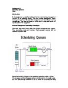
Here we can see that the process number one is dispatched from the ready queue and enters the processor straight away. The process need not wait as it is the first to enter. The process takes 24 seconds to complete by which time the processes 2 and 3 are ready and waiting, this take’s up to 30ms. The average waiting time is then calculated as follows
(0 + 24 + 27) / 3 = 17ms
As previously said this time can be considerably reduced if the order is reversed. Here is the average waiting time if the processes are reversed.
(6 + 0 + 3) / 3 = 3ms
This is a significant improvement and reduces waiting time dramatically. Looking at the figures above it comes as no surprise that this method is rarely used in a day to day environment.
Shortest Job First
The processor will execute each job in order of the completion time from lowest to highest. However; the first job received in the processor will be executed first even if it’s bigger than any of the others in the queue. This method can reduce time and is far more efficient than FCFS. It can only work though if the CPU is aware if each processes burst time and then when this is achieved order can be obtained. This is a form of processing scheduling which has the lowest average waiting time using its algorithm. It’s also a very clever processing technique. The processor cannot actually define the burst times individually so the operating system takes into account the previous burst times and then makes an average. This is a very clever feature.
0 7 8 12 16
Average waiting time = (0 + 6 +2 +7) / 4 = 3.75
Shortest Remaining Time First
This form of processing method will ensure that each process entering with the shortest remaining time will be completed first. This then allows the processor to hand out interrupts until the scheduling is completed. This processing method however has a very big problem. What is to say that every job that will enter the processor will be a short one? The problem is starvation for longer jobs. The only time the processor needs to reschedule is when a new process arrives in the ready queue with a shorter time than the current process, if this is the case then the current process is put into the ready queue and swapped concurrently. Since this is the only time when a process need be switched, it results in much less overhead than the Round Robin technique that I will describe next.
0 2 4 5 7 11 16
Waiting times: P1 = 9, P2 = 1, P3 = 0, P4 = 2
Average: (9 + 1 + 0 + 2) / 4 = 3
Round Robin
This processing technique is the most complex of the four studied. It can be compared to FCFS for the pre-emptive abilities to switch between processes. Each process is give what is known as a quantum; this can be a time period of 10 to 100ms. Each process then cannot exceed the quantum within the processor. The ready queue is now made into a round queue and anything exceeding the quantum will be put at the back with the head process taking priority of the queue. When exceeded, the process shall be placed at the back of the queue and will be given an interrupt. It can be said that the round robin technique is a fair one.
- If there are n processes in the ready queue and the time quantum is q then each process gets 1/nth of the CPU.
- No process waits more than (n-1)q time units before receiving CPU allocation
- It typically has a higher turnaround time than SRTF but a better average response time.
The table below works on the basis of a time quantum of 4ms.
0 4 7 10 14 18 22 26 30
Above can be seen a time quantum dictating the length of a process in the CPU. It can be said for definite that the process cannot exceed the quantum even if their are no other processes in the queue. We can also see that the P1 uses a whole time quantum; P2 and P3 however only use a part of it.
P1 waits 0 + 6 = 6, P2 waits for 4 and P3 waits for 7
Average time = (6 + 4 + 7) / 3 = 5.66ms