Modelling is about building representations of things in the ‘real world’ and allowing ideas to be investigated. It is central to all activities in the process for building or creating an artifact of some form or other. In effect, a model is a way of expressing a particular view of an identifiable system of some kind. Models are, in one respect, idealizations in the sense that they are less complicated than reality, they are simplifications of reality. The benefit arises from the fact that only the properties of the world relevant to the job in hand are represented. For example, a road map is a model of a particular part of the earth's surface. We do not show things like vegetation or birds' nests as they are not relevant to the map's purpose. We use a road map to plan our journeys from one place to another and so the map should only contain those aspects of the real world that serve the purpose of planning journeys. One of the simulator software is the STELLA software. STELLA offers a practical way to dynamically visualize and communicate how complex systems and ideas really work. STELLA models enable us to communicate how a system works like what goes in, how the system is impacted, what are the outcomes.
STELLA supports diverse learning styles with a wide range of storytelling features. Diagrams, charts, and animation help visual learners discover relationships between variables in an equation. Verbal learners might surround visual models with words or attach documents to explain the impact of a new environmental policy.
The purposes of STELLA usage are to stimulate a system over time, jump the gap between theory and the real world, enable students to creatively change systems, teach students to look for relationships and clearly communicate system inputs and outputs and demonstrate outcome.
The example of the sample model that can be found in the STELLA website is pendulum story. A simple pendulum is one which can be considered to be a point mass suspended from a string or rod of negligible mass. It is a resonant system with a single resonant frequency. A simple pendulum consists of an object suspended by a string of length l. The bob swings back and force. The gravitational force, the weight (W), is resolved into two components. The parallel component is along the direction of the spring. The perpendicular component is at right angles to the direction of the spring. When the bob is pulled to the right, the perpendicular component is to the left, and vice versa. That is, the component of the weight (perpendicular), is a restoring force. Further, for small angles (less than 15°) the magnitude of perpendicular component is proportional to the displacement of the bob. Thus, small-displacement pendulum motion is an example of simple harmonic motion. The time for one complete cycle, a left swing and a right swing, is called the period. A pendulum swings with a specific period which depends (mainly) on its length. When given an initial push, it will swing back and forth at constant amplitude. Real pendulums are subject to friction and air drag, so the amplitude of their swings declines. The period of swing of a simple gravity pendulum depends on its length, the local strength of gravity, and to a small extent on the maximum angle that the pendulum swings away from vertical, θ0, called the amplitude. It is independent of the mass of the bob. If the amplitude is limited to small swings, the period T of a simple pendulum, the time taken for a complete cycle. For small swings the period of swing is approximately the same for different size swings: that is, the period is independent of amplitude. Successive swings of the pendulum, even if changing in amplitude, take the same amount of time. For larger amplitudes, the period increases gradually with amplitude.
There are three different types of oscillation that are free oscillation, damped oscillation and fixed oscillation. Free oscillations occur while the pendulum is sets to its displacement and is moving in its to and fro motion it does not experience any force that prevents it from continuing this motion. Such forces that prevent free oscillation is air resistance. Damped oscillations occur while the pendulum is set to its displacement and is moving in it to and fro motion, experiences a force, or a medium that affects its motion. A forced oscillation occurs while an object is used to force or more pendulums into motion. An example of this is by using a driving pendulum to control the displacement of a set of 4 pendulums, which move as a result of the driving pendulum being displaced. Other than that, the other example is using a vibrating tuning fork to force a stretched string to vibrate and set the pendulum into motion. The simple gravity pendulum is an idealized mathematical model of a pendulum. This is a weight or bob on the end of a massless cord suspended from a pivot, without friction. When given an initial push, it will swing back and forth at constant amplitude. Real pendulums are subject to friction and air drag, so the amplitude of their swings declines.
Picture 1: the front page of the pendulum sample in STELLA
This software is a shareware type of software. So, we need the license to use this software. As the trial, we are given free trial version that will time out 30 days after the installation. We need to register at the website to download the software. The picture above is the free trial version of STELLA. By using STELLA software, the student can relate the result of the simulation to the theorem of simple pendulum. This is because the can varied the variable that affect the experiment such as mass of the bob, string length, initial displacement, air friction and driving force. In the task given by Encik Azmi to us, we need to find discuss about three variables that affect the experiment we choose to use in the STELLA software. By using the STELLA software, my variables are string length, initial displacement and mass of the bob.
Picture 2: the oscillation of the pendulum at the normal condition
Picture 3: change of mass of bob
Picture 4: changes of initial displacement of bob
Picture 5: changes in length of string
At the STELLA software, we click the button “conduct experiments” to begin the experiment of the simple pendulum. From picture 2, I choose the normal condition to be a guideline to compare with latter experiments. As the guideline, I fixed the mass of the ball is 1.0 kg, initial displacement is 0.1 m, and the string length at 1m. By put the normal condition oscillation together with the graph that I change the parameter, I can compare directly to make the analysis of the experiment. All the experiment that I done is only under the gravitational force and not include the air friction and drive force. The first parameter I change is the mass of pendulum. From picture 2 above, graph 1 is the oscillation at normal condition (mass=1kg, initial displacement=0.1m and string length=1.0m), graph 2 at the mass of pendulum is half the initial mass of pendulum of normal condition (mass=0.5kg, initial displacement=0.1m and string length=1.0m) and graph 3 is the pendulum with double mass of the pendulum at normal condition (mass=2.0kg, initial displacement=0.1m and string length=1.0m). So, from the graph, we see that all the graph have the same frequency, amplitude and period. This situation shows that the mass does not affect the oscillation of pendulum. To find the period of oscillation of the pendulum, we use
And we found that the mass not one of the parameter that change the period of oscillation. So, the graph in picture 2 proves the equation. From the picture 3, I simulate the oscillation at different initial displacements. Graph 1 is at normal condition that will become the guideline of other graph, graph 2 is the pendulum with initial displacement of 0.15m and graph 3 with initial displacement of 0.2m. From the graph, we can see that the frequency of all graphs is same with each other and different with the amplitude of the graph. When the initial displacement increase, the height of displacement also increases, the potential energy increases, so kinetic energy also increase but the time period remains same.
Next, the parameter change is the length of string of the pendulum. From the picture 3, we have the graphs. Graph 1 is the oscillation at the normal condition (mass=1kg, initial length=0.1m and length of string=1.0m), graph 2 with the length of string is half than the length of string at normal condition (mass=1kg, initial length=0.1m and length of string=0.5m) and graph 3 at the condition where the length of string is double the normal length of string of pendulum (mass=1kg, initial length=0.1m and length of string=2.0m). From the picture 3, the amplitude of all graphs is same but different with the period of oscillation. The period of oscillation is increase directly with increasing the length of the string of pendulum. From the equation period of oscillation that I stated above, length of string a factor that changes the oscillation of pendulum. The obtained graphs prove that equation. As a conclusion from the experiment, there are two factors that affect the period, frequency and amplitude of the pendulum. In this case, initial and length of the string affect the period of oscillation, frequency and amplitude of the pendulum while the other parameter that is mass of the ball do not affect the motion of the pendulum.
By using STELLA software to conduct the experiment, we can see that the data obtained is very accurate. For example, if we conduct the experiment of pendulum with different masses manually, we barely get the expected data and graph like picture 2. So, by using the STELLA software, the student able to do the experiment without making mistakes and able to relate the experiment with the given equation of pendulum.