P =
Table 2: First estimate for Case 1
Due to the inaccuracy, the first estimate was obviously wrong. Adjusting the numbers is necessary:
P = +
Table 3:Second Estimate for Case 1
Although this is still quite a large difference, it is much closer to correct than the first estimate, maybe one more will get close enough:
P = +
Table 4:Third Estimate for Case 1
This formula is a good representation of the relationship between Payoff and Odds of winning for the Lotto 649 Lottery.
Case 2
The game of chance that is mentioned in the St. Petersberg Paradox involves a fair coin. It is repeatedly tossed until, on the nth toss, the coin lands heads up. The payoff is $. Entry to the game shall be set at $5 for the purposes of this essay. Below is a tree diagram of the game:
H T
But because there is no theoretical end to this game, the expected value has no theoretical limit either as shown:
+…++…=
Thus, the expected value tends towards infinity as number of trials increases towards infinity. However, on any one trial, it is much more likely to lose money instead of making infinite profit.
If it is considered that when P• E, one has lost money, one has the infinite sum of the geometric sequence odds of making money with this game.
Sum to infinity = when a is the first term in the sequence, and r is the ratio between terms. Thus = one has a 1 in 4 chance of making money when paying a $5 entry price. When compared to Case 1 and its odds of making money this game seems quite good. To make the games equal in odds, the entry price to Case 2 must be raised substantially: when a is the reciprocal of the entry price(the odds). Here a comes to equal which implies that the entry price would have to be in the range from $131073 and $262144 . This price seems outrageously large and that gives a sense of the odds involved in playing the lottery, yet 4 million tickets are sold for lotto 6/49 every week on average.
Case 3
The third game is the Heart and Stroke Lottery from the Heart and Stroke Foundation of Ontario. Entry is $100 a ticket, and there is a set limit of 222 000 tickets sold. For the purposes of the calculations, all of the prizes from $1 000 000 to $22 207 shall be ignored. This is because the Payoff and the Odds are quite incongruous throughout these prizes. The reason for this, without delving too deeply into macroeconomics, is incentives. (Attached in the appendix is a complete list of prizes) Tickets are drawn from the 222 000 at random and the payout scheme is below:
Table 5: Data for Case 3
But all of the prizes shall be included when calculating the expected value (except the values of all of the cars shall be added together for presentational purposes) thus expected value =
++
++
= -$66.6499414414
The odds of winning anything are
Payoff is inversely proportional to the Odds of winning, as shown below: Fig. 3:
Once again, a process of regression will be used to find the function of the relationship between Payoff P and Odds of winning (O). Because the data points look to the naked eye as if there could be a linear relationship, my first estimate will be linear in nature, or be in the form:
P =
Table 6: First Estimate for Case 3
But since it does appear to have a slight curve, perhaps a quadratic equation would be more accurate:
P = +
Table 7: Second Estimate for Case 3
This is an improvement on the linear equation, and it is a good representation of the data.
Comparison
A major difference between these three games is the entry price. In the lotto 649 lottery, it is a relatively small $1, with a possibility of winning $2 000 000. The Heart and Stroke Lottery has a somewhat higher entry price of $100, and the most one stands to win is $1 000 000. Admittedly, one is approximately 136 059 times more likely to win the
$1 000 000 prize, but is it worth the extra $99 of entry fees? Similarly, if the three games’ chances of winning anything are compared versus their entry price:
Table 8: Comparison of games by odds
When considering entry price E, its value depends on two things, odds of winning and potential payoff. It is clear in case 1 that the very low entry price is not paying for good odds, but instead it pays for large potential winnings. Case 2 has a larger entry price, and this increase makes the odds much more favourable. Case 3 is the truly interesting example though because the entry price is now $100, a great deal more expensive than either of the other two games. The effect of this high entry price is not only quite favourable odds, but also still a lot of money to be won.
If the above functions were used to predict odds of the three games at certain levels of payoff, it would show which games are more favourable in different situations.
When P = $500 000:
Case 1
P = +
=
OR, O =
Case 2
P =
O =
Case 3
P = +
OR, O =
When P = $100 000 000
Case 1
P = +
=
OR, O =
Case 2
P =
O =
Case 3
P = +
OR, O =
When P = $5 000
Case 1
P = +
=
OR, O =
Case 2
P =
O =
Case 3
P = +
OR, O =
These calculations are summarized in Table 9:
Table 9: Using found functions to estimate odds
To find which game is the best one to play for different levels of payout, the intersection of the functions must be found. Between case 1 and case 2, where
P = + and P must also = , P can be substituted in for every so the equation will be PPP + 27
P =
P = 52 631 421 052 600 and P = 27
P = 27 is a fault of the function used because it misrepresents the curve at small values of P, Case 2’s odds of winning are better than Case 1’s until the payout of the games reaches $52 631 421 052 600, but this situation is unlikely to occur because of its size. To compare Case 2 to Case 3, the intersection of their functions must be found; thus P = , and P = + . Once again, will be substituted for P: P = P+ + 78
P =
P = 822 505 and P = 95
P = 822 505 is once again an error of the function chosen. Because the function was based upon the smaller numbers, one can expect that the function will become inaccurate past these numbers. Case 3 is a better game to play for payoffs less than $95. Finally when comparing Case 1 to Case 3, the intersection of their functions must be found, so
P = + and P = +
When these equations are set as equal a quadratic in the reciprocal of the odds is formed:
9.99999981= 0
This quadratic however has no positive roots; this is because Case 3 is always a better game to play when only considering the odds. But it must be recalled that the function found to represent Case 3 was based on smaller numbers, thus it is misleading to compare it to other cases.
These three games do encompass most of the variables involved in gambling. They have been examined and analyzed thoroughly to show relations between the three major variables, P, E, and O. I have made some conclusions based upon my observations; firstly, secondly that E. Thus every game of chance which involves these three variables revolve around the same proportionality:. Therefore, the payoff of a game must be equal to a constant c multiplied by the entry price divided by the odds, or. I theorize that the magnitude of this constant c determines the attractiveness of games of chance. After finding the odds of the lotteries, I do wonder why people spend their money on them; it is simply a voluntary taxation in my opinion. Another question that arises is, if someone were to run a business based on the game used in Case 2, would it be profitable? And at what price would people be willing to enter, even though mathematically it has no bearing on their long term success in the game?