Revised set of sample data
This is set of sample data is going to be used through out my investigation of the length of the line.
I will now begin my investigation.
Firstly, I will begin by converting all the line and angle data points into their percentage errors. As said in my plan, this is done to implement a clear comparison.
I will first need to work out all the errors of the data points. We do this by subtracting the just the original guesses from the correct length of the line and size of the angle.
I will use Excel to help me with this as through the use of excel we can use simple formulas to work out equations.
Testing the hypothesis
The hypothesis states that people estimate the lengths of lines better than the size of angles. I will now test this hypothesis by calculating the mean and of both line results and angle results and compare them. Once I have done this I will then implement other methods, such as standard deviation cumulative frequency graph, and inter-quartile range.
Comparing data
As I mentioned earlier, we need to be able to compare the line an angle guesstimate data, but at the moment there is no comparison. To be able to compare this data we need to find a comparison. The best comparison is to work out the percentage errors for each line guesstimates, and angles guesstimates, as this is relevant to both the two different units of measure and will be easy to compare.
First thoughts and assumptions
I think from what I know about angles and lines that the hypothesis is wrong and that people will estimate the size of the angle more accurately.
When considering the length of a line its difficult to know just how long it is, this is because an exact line length is difficult to visualise, whereas with an angle we know that 90 degrees is a right angle, 180 degrees is a half, and this we can picture in our minds. So when we see an angle we use the visualisations of sizes of angles that we know to be true to estimate the size of another angle, as they have to be either smaller or bigger than these. But when we try an estimate the length of a line it’s not so easy, as a line has no limitations, it can be as long as we want, but an angle can be no greater than 360 degrees. Also an angle is a fraction of a circle, but a line can be a fraction of a line than has an unimaginable greatness of length.
So baring this in mind, when people estimate the size of the angle I think they will be closer to the correct size, than when they estimate the length of a line.
Calculating the percentage errors for line guesstimates
I will start by investigating the line.
I first calculated the errors, by subtracting the correct length of the line away from the guesses. Once I had calculated the errors I was then able to use the percentage error formula:
Error ÷ Correct × 100
= percentage error
In excel we do this in the percentage error column by dividing the first data point in the line error column by 45, then by multiplying this by 100 to find the percentage.
This found the percentage error for the first data point, to find the percentage error for all the other data points, because the formula is the same for each of the other data points in this column we simply highlight the first data point using the right click of the mouse, drag down and the formula works out the percentage error in each cell.
Calculating the percentage error for angle guesstimates
When calculating the percentage error for the angle guesstimates, we repeat the same process needed to work out the percentage errors for the line guesstimates. Except in this case we divided the errors by 36, as this was the correct size of the angle.
Now that I have calculated the percentage errors for all data points of line and angles within my sample data, I will be able to proceed with my fist method of proving or disproving the hypothesis, this will be by calculating the mean of line percentage errors and angle percentage errors. I will then compare both means.
Calculating the mean of the line percentage errors
To calculate the mean percentage error, we need to use the usual method of calculating any mean result. We need to add up all the percentage error data points and divide by how many data points there are. But before we can do this we need to make any negative percentage error data points positive. If this is not done, when we add up all the data, the negative data will subtract itself from any positive data, and this we do not want, as we are only looking at the percentage of which they were away from the correct, weather or not the guess was too high or too low, is insignificant.
Adding all percentage errors
To add the percentage errors we need to convert the negatives into positives, as said earlier. I did this in excel by squaring each negative percentage, by using the formula ^2, and then square rooting each percentage. Once I had done this I was able to add up all the percentage errors by first highlighting all the data points in the percentage error column and then by using the formula ∑ in excel, which means the sum of. This gave me the sum of all the percentage errors for the line, and the angle. The sum of the percentage errors for the line was 981.5555556% and for the angles 795%.
Finding the mean percentage error
What I did next was divide both numbers by 40, as this was the amount of data points. I was left with the products, 24.53888889% for the line, and 23.625% for the angles, which were the mean percentage errors. These are highlighted in yellow.
The hypothesis states that people estimate lines better than angles. From information I have gathered through calculating the mean result of the percentage errors I have found that my findings contradict the hypothesis, and that people tend to estimate the size of angles better than the length of lines. My assumption that people will estimate the size of the angle better than the length of the line, for reasons mentioned earlier, was found to be true through this investigation.
If I were able to make these findings more reliable I would have sampled a larger amount of data from a more extensive pool of data, as this would have decreased the effect that unreliable, bias data had on the mean.
I will now investigate through other methods of proving and disproving the hypothesis.
Cumulative frequency
I could have at this point produced a frequency graph, but due to limitation in time I have decided to produce a cumulative frequency graph as this is a clearer, indicative representation of data, and I will be able to deduce more information from it.
If we represent the percentage errors of both line and angle percentage errors individually in frequency tables, we can calculate cumulative frequencies. Once we have done this we can use these new values, when plotted and on a graph, to form a cumulative frequency curve. This is useful as we will be able to find the median from the halfway point, and we will be able to locate the upper and lower quartiles.
The upper quartile is 75% and the lower quartile is 25 %. From knowing the upper and lower quartile, we can calculate the inter-quartile range. This is found by subtracting the lower quartile from the upper quartile. The inter quartile range is half of the data distribution and shows how widely spread the data is, if the inter-quartile range is small, then the distribution is bunched together and shows more consistent results, if the inter-quartile range is large, then the distribution is spread and shows a wider variation in results.
We can compare both the line inter-quartile range and the angle inter-quartile range, and whichever is smallest, will be the most accurate, as this would mean a smaller percentage error.
Line percentage errors cumulative frequency table
To produce a cumulative frequency table, you first set the boundaries for each group of percentage errors this has been done in the first column. We then count all the percentages that are within the boundaries of that group, and this is then recorded in the frequency column. Once this has been done for each group, we can then calculate the cumulative frequency by adding each of the previous frequency data points to the next, and record each product in the cumulative frequency column. We then state in the in the upper limits column, what the highest percentage error can be.
Now that I have produced a cumulative frequency table, I can now start to produce a cumulative frequency graph.
Line percentage errors cumulative frequency graph
The graph shows the cumulative frequency curve of the line percentage errors. From this curve I can find the lower and upper quartiles. These were;
Lower quartile = 13%
Upper quartile = 35%
From knowing the lower and upper quartiles, I can calculate the inter-quartile range, by simply subtracting the lower quartile from the upper quartile.
Inter-quartile range = (35 - 13) % = 22%
The inter-quartile range of the line percentage error, cumulative frequency graph is 22%.
I will now investigate the cumulative frequency graph, of the angle percentage error.
Angle percentage errors cumulative frequency table
I have produced the cumulative frequency table for the angle percentage errors. I can now begin to draw the cumulative frequency graph. Once I have drawn this I will calculate the lower and upper quartiles, and then calculate the inter-quartile range. Once I know the inter-quartile range I will be able to compare the inter-quartile range for the line data and the inter-quartile range for the angle data
Angle percentage errors cumulative frequency graph
The graph shows the cumulative frequency curve of the angle percentage errors. From this curve I can find the lower and upper quartiles. These were;
Lower quartile = 12%
Upper quartile = 28%
From knowing the lower and upper quartiles, I can calculate the inter-quartile range, by simply subtracting the lower quartile from the upper quartile as I did for the line percentage cumulative quartiles.
Inter-quartile range = (28 - 12) % = 16%
Comparing graph data
I have found the inter-quartile range of both line and angle cumulative frequency graphs. Theses were, for the line percentage errors- 22%, and for the angle percentage errors-16%.
It’s clear to see from these results that the inter-quartile range of the angle percentage errors was much less than the inter-quartile ranges of the line percentage errors. There is a difference of 6% percent between the two results. This shows that there was a wider spread of data for the line percentage errors, and that the accuracy when estimating the lines length was not as precise as when the angles were estimated.
I have shown through my investigations that when people estimated the length of a line and the size of an angle, results were more accurate when the size of the angle was estimated. My first thoughts were that people would estimate the size of angles better, as angles are a fraction of a circle, which is limited. But the length of a line is un-limited and it is difficult to visualise the correct length of lines. I believe that my thoughts could be true as the mean and inter-quartile range of the angle percentage errors, were more accurate than the line on both occasions. I have investigated this hypothesis using two different methods, and through them have concluded that people estimate the length of angles more accurately. My findings contradict the given hypothesis.
Now that I have finished investigating the given hypothesis, I will begin to investigate my own hypothesis.
Hypothesis 2
“Females estimate the length of lines and size of angles better than males”
The above hypothesis is a hypothesis of my own and is one which I will now begin to investigate. I will use the same method of comparing percentage errors as used in the previous investigation.
First thoughts
Without analysing the comparisons between the results given from the different sexes, it’s difficult to say weather or not females were more accurate, as at first glance, it is not obvious.
Data analysis
To be able to compare male and female estimates, I must first divide my sampled data into two sections, one section of male estimates and another section of female estimates.
Earlier in my investigation I specifically selected 20 male data points and 20 female data points using ‘Stratified random sampling’, to eliminate bias. This is now useful to me as than there is an equal amount of female and male data points, so I will be able to use an analyse my original set of sampled data. I will now separate male and females guesses into two columns and compare the mean of the percentage errors.
I will be able to mix line and angle percentage errors as I am comparing how females and males estimate lines and angles generally and not line and angles individually.
Male Line and Angle percentage errors
To calculate the mean percentage error I first need to add up all the percentage errors. To do this, I will use the ∑ formula in excel, as used earlier.
The number highlighted in green is the sums of the line and the angle percentage errors. To gain the mean of the percentage I need to divide them by 40, as this is the amount of percentage error data points.
The product I am left with is 23.70833% this is the mean percentage error for male line and angle estimates.
Female Line and Angle percentage errors
If I repeat the same process used for the male percentage errors, to obtain the mean of the female percentage errors, I am left with the product 26.41667%. This is the mean percentage error for line and angle percentage errors.
From calculating the mean percentage errors of line and angle percentage errors, for both genders, I have found that males were more accurate at estimating the size angles and length of lines than females, and that this contradicts my hypothesis. To improve the reliability of my findings I will now investigate standard deviation.
Standard deviation
Standard deviation is useful to measure the spread of the data. Standard deviation gives a more detailed picture of the way in which data is dispersed around the mean, being the centre of distribution. If the difference between the standard deviation and the mean is large, the data is not consistent and is not typical of the mean.
To work the standard deviation, I need to subtract the mean percentage error from each percentage error to create a set of deviations. Once I have done this I need to square each deviation to make a set of squared deviations.
I can place this information in a table
x = percentage error
x = mean percentage error
I then need to average the set of deviations, by finding the mean of the standard deviations. Once I have done this I will need to take the square root so that the answer is back to the original measure, in this case percentage.
This can be represented by the formula √ ∑(x - x) ² ÷ n
I will now use my male sample percentage error data, to formulate a table
Standard deviation table of male percentage errors
Once I had organized the data from smallest to largest in column x, I could calculate column 2(x-x) by subtracting the mean, which is 23.70833, from each percentage error. I then calculated column three (x-x) ² by multiplying each data point in column two by power 2, by using the excel formula ^2.
Calculating the Standard Deviation
Once I had finished formulating the table, I was able to find the Standard Deviation. I need to use the formula √ ∑(x - x) ² ÷ n. So I firstly had to work out the sum of the (x-x) ² column, the product was 13045.912. I then divided this number by 40, to find the mean of the data, as this is the number of data points and the product was 326.14781.The final calculation I had to make to conclude with the standard deviation was to square root the mean, as I needed to find the original unit of measure, in this case it was percentage.
The standard deviation of the male line and angle estimates is 18.1% to 3.sf.
Standard deviation table of female percentage errors
Once I had organized the data from smallest to largest in column x, I could calculate column 2(x-x) by subtracting the mean, which is 26.41667 from each percentage error. I then calculated column three (x-x) ² by multiplying each data point in column two by power 2, by using the excel formula ^2.
Calculating the Standard Deviation
Once I had finished formulating the table, I was able to find the Standard Deviation. I needed to use the formula √ ∑(x - x) ² ÷ n. So I firstly had to work out the sum of the (x-x) ² column, the product was 13045.912. I then divided this number by 40, to find the mean of the data, as this is the number of data points and the product was 326.14781.The final calculation I had to make to conclude with the standard deviation was to square root the mean, as I needed to find the original unit of measure, in this case it was percentage.
The standard deviation of the male line and angle estimates is 25.8% to 3.sf.
Comparing data
From investigating my hypothesis, I have found that through investigating the mean of the percentage errors for male and female estimates, males were more accurate. But when I investigated the percentage errors through standard deviation, I found that females were more consistent with estimating and that female estimates were more typical of the mean than male estimates. But this is irrelevant as the data still shows that males were more accurate as the standard deviation of the male estimates was 18.1% and the standard deviation of female estimates was 25.8%, which is a difference of 7.7%. My findings contradict my hypothesis and males were more accurate at estimating lengths of lines and size of angles.
Evaluation
I believe that I have investigated both hypotheses as much as I could have in the time I have been given. The conclusions I have come to through my findings were based upon the data pooled by my class. I believe that some of this data may have been unreliable due to errors etc. I believe that with a more extensive pool of data, my findings would have been more conclusive an indicative a true representation.
I have reached the end of my investigation. If the time allocation was greater, I could have investigated another hypothesis such as “Younger people estimate lines and angles better than older people”.
STATISTICAL COURSEWORK
GUESSTIMATE
COURSEWORK
Khalil Sayed-Hossen 10B