Table of Values
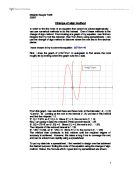
The graph does not display any change of sign, implying that there are no roots. However, it is evident from the graph that there are two roots (see magnified version of graph). However, as the two roots are so close together, the decimal search method does not detect this and so in this instance, this method cannot be used to help solve the equation y=0.6918x3 – 0.2159x2 – 3.019x + 2.77
Newton Raphson Method
Using this method, a first approximation, x1 is made. The intercept of the tangent at (x1,y1) with the x axis is found as the next approximation, x2. This process is repeated until the desired accuracy is achieved. This method is also known as the ‘Tangent Sliding’ method.
This method can be demonstrated manually, using the equation: y= 20x3 + 15x2 – 15x – 12
F (x) = 20x3 + 15x2 – 15x – 12
F’(x) = 60x2 + 30x – 15
First estimate x1 will be 1
First iteration
F (1) = 20(13) + 15(12) -15(1) – 12 = 8
F’(1) = 60(12) + 30(1) – 15 = 75
X2 = 1 – 8/75
X2 = 0.8933
Second Iteration
F (0.8933) = 20(0.89333) + 15(0.89332) – 15(0.8933) – 12 = 0.82906074
F’(0.8933) = 60(0.89332) + 30(0.8933) – 15 = 59.68266667
X3 = 0.8933 – 0.829/59.68266667
X3 = 0.879442165
X3 = 0.8794
Third iteration
F (0.8794) = 20(0.87943) + 15(0.87942) -15(0.8794) – 12 = 0.01318348
F’(0.8794) = 60(0.87942) + 30(0.8794) – 15 = 57.78837624
X4 = 0.8794 – 0.013/57.79
X4 = 0.879214031
X4 = 0.8792
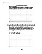
This can also be demonstrated graphically using the computer programme autograph:
y= 20x3 + 15x2 – 15x – 12
First iteration
X = 0.8933
Second iteration
X = 0.8794
Third Iteration
X = 0.8792
The results have converged to 0.8792
To confirm that this is a root by looking for a change of sign
F (x) = 20x3 + 15x2 – 15x – 12
F (0.8791) = -6.5827 x 10-3 = negative
F (0.8792) = positive
Therefore the root is 0.87925 ±0.00005
Where the method cannot work
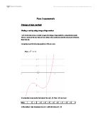
If the initial estimate is too far from the required root, the method can fail.
This can be shown using the equation y=20x3 + 15x2 – 8x – 19
Take the initial estimate as x1 = -1
First Iteration
x = - 0.2727
Second Iteration
x = -1.647
Third Iteration
x=-1.13
Evidently, this method fails in this instance. However, the use of a sketch graph can avoid these problems.
Graphical Convergence
This method can be used if f(x)=0 can be rearranged to give x=g(x). a first approximation x1 to the root is made and an iterative formula is used successively until the desired accuracy is achieved. This method is also known as the ‘staircase method’.
This can be demonstrated using the equation y=x3 – 4x +1
Solve x3 – 4x+1 = 0
The equation is initially rearranged into the form x = x3 + 1 = g(x)
4
This can be used as the iterative formula xn+1 = xn3 + 1
4
The initial estimate of the root is 1
x1 = 1
x2 = 0.5
x3 = 0.28125
x4 = 0.25556
x5 = 0.25417
x6 = 0.25411
x7 = 0.25410
x8 = 0.25410
The root appears to be 0.25410
To confirm that a root has been found, we need to look for a change of sign.
F(0.25411) = -0.000031637 = negative
F(0.25410) = 0.000006426421 = positive
Therefore the root is 0.254105 ± 0.000005
This can be demonstrated using the graph:
First Iteration:
Second iteration:
Sixth Iteration:
The roots of x=g(x) are the values of x at the points of intersection of the line y=x and the curve y=g(x)
The reason this works, is because the gradient of the curve at the required root is less than 1.
Where this method does not work.
If the initial equation is incorrectly rearranged, it may lead to convergence to the wrong root, resulting in the method not working.
For example, if the equation, y= x3 – 4x+1, is incorrectly rearranged, so instead of x = x3 + 1
The equation is rearranged to x = 3√4x-1. 4
Using the graphical convergence tool on Autograph, attempts to find the root can be easily carried out, taking the initial estimate as x1=2.
As the graph displays, this incorrect rearrangement of the initial equation has not lead to the convergence of the required root. However, it continues infinitely upwards, as shown below:
Comparison of methods
To investigate the usefulness of each method, comparisons can be carried out. This can be done with the previously used equation y = x3 – 4x+1
Decimal search
First interval
The table shows that the sign changes within the interval 0.2 to 0.3. This tell us that the roots lie somewhere within this interval;
Therefore the root is 0.25 ± 0.05
Second interval
The table shows that the sign changes within the interval 0.25 to 0.26. This tell us that the roots lie somewhere within this interval;
Therefore the root is 0.255 ± 0.005
Third interval
The table shows that the sign changes within the interval 0.254 to 0.255. This tell us that the roots lie somewhere within this interval;
Therefore the root is 0.2545 ± 0.0005
Therefore, using decimal search, we can see that the root found is 0.254, as this is where the sign changes from positive to negative.
Newton Raphson Method
First Iteration:
x = 0.25
Second Iteration
x = 0.2541
Therefore, using the Newton Raphson method, the root has been found to be 0.2541
Using the graphical convergence method, the root has already been found to be 0.2541.
Comparisons
Whilst all methods give similar answers, some methods are more beneficial than others.
The Change of sign method is easy to understand, and error bounds are easy to find at each stage, which allows us to know the accuracy of the final result. However, if a high degree of accuracy is required, this method can be laborious. Furthermore, if there are a number of roots close together, or there is a repeated root, the method can fail. Also, this method cannot deal with a non-continuous function such as f(x) = 1/x
Whilst the Newton Raphson method allows quick convergence, and is easy to perform on autograph, the method could be criticised, as it requires calculus, unlike decimal search. It can also be subject to failure, for example, if the initial estimate is made too far from the required root. Furthermore, to find an error bound for increased accuracy, decimal search needs to be carried out, again adding to the amount of work required. This disadvantage can also be applied to the graphical convergence method. In this method, there is also a high failure rate, as it can diverge, oscillate or converge to the wrong root, as shown in the calculations. Also, you may not be able to rearrange f(x) =0, in which case this method could not be used.
Therefore, in conclusion, whilst each method can be used to find roots, a d=sketch of the graph should be drawn, before deciding upon which method will work the best, and the level of accuracy that is desired.