Error bound: ±0.000000005 (9dp)
The table below shows part of the formulas used in the Excel.
Failure in this method
This method cannot always be applied to every equation successfully. For example in the following case:
Equation A:
→
The graph above shows us that the roots of the equation are very close. Zoom in on the x and y axes, we can see that they all lie between x=0 and x=1. Use Autograph that follows the same steps as Equation 1 we can only get one of the three roots, which is shown below graphically.
Using Excel, if we start the interval with x=0 and x=1 and follow the same steps as done in Equation 1, we end up with only one root.
Since this method cannot find out all the roots, we say that it fails in this case. For the example above, it is because the three roots lie too close together. We usually ignore the other two roots when we find out one in the interval since we didn’t expect them all in such a small interval.
Method 2: Newton-Raphson method
Equation 2:
→
Here shows the overall view of the graph of the function.
Zoom in on the axes we can clearly see that using the Newton-Raphson method gives us one root efficiently.
How does the Newton-Raphson method actually work?
The graph above shows a part of a function (the blue curve). Suppose we have an estimated value of a root, xn. Draw a tangent at where x=xn, which is shown in red, we can get another estimated root xn+1 which is a better approximation.
Since, we can deduce that.
With the help of Excel, we can get the approximate value of the root shown above within just a few steps.
The table below shows the data with accuracy of 8 decimal places.
And here’s the formulas used in the table:
Similarly, starting with another two points, we can get the approximate values of the other two roots. The tables below show the data with accuracy of 8 decimal places as well.
The approximate values of the three roots are 0.19806226, 1.55495813, and 3.24697960 (correct to 8dp).
Error bounds: ±0.000000005 (9dp)
Failure in this method
However, sometimes we may want to find a particular root by using this method but it occasionally fails and finds another one.
Here is a counter example:
Equation B:
→
Here gives the overall view of the graph of the function.
Zoom in on the axes and we can see that there is a root lying between x=0 and x=1. Supposing we want to find this root, we might consider starting at x=0 since it is quite close to the root.
Since the gradient at x=0 is very small, the tangent diverges from the root and finally finds another root near x=6 which is not the solution we expect. So, although we start with a value that is quite close to it, we fail to find the particular root we want. That is why the failure occurs.
Method 3: Rearrangement
This method aims to rearrange f(x)=0 in the form x=g(x) and hence find the intersection points of y=x and g(x). The corresponding x values are the roots of f(x)=0.
Equation 3:
Rearrange the equation, let
→
→
Use Autograph to draw the graphs of and.
We can see from the graph that the method leads us to one root efficiently.
By adding the original equation (the red one) to the graph, we can see that the x values of the intersection points are the exactly same as the roots of the original equation.
As in the example above, we want to find the root which lies between x=0 and x=1. In this case we might consider a starting point of x=1. Excel can help us with the process of getting the approximate value of the root.
The table above provides us with data accurate to 8 decimal places and it shows that the approximate value of the required root is 0.40303172.
From the table we can see that |g’(x)| ≤1.
Error bounds: ±0.000000005 (9dp)
The formulas used are shown in the following table:
Failure in this method
However, if we rearrange the equation in another way, we might not get the same results as we expect.
Let
Use Autograph to draw the graph of and.
Suppose we want to find the root that lies between x=-1 and x=0. With a starting point at x=-1, we can see that it finally diverges away from the required root and enters a recursive cycle.
The Excel table above provides us with data accurate to 8 decimal places. From it we can see that |g’(x)|>1.
Comparing the two examples above, we can deduce that when |g’(x)|≤1, it converges to the root and we are able to find the value of it and when |g’(x)|>1, it seems to diverge from the root and the failure occurs.
Comparison of 3 methods
In order to compare the above 3 methods, choose Equation 3 and apply it to the other two methods.
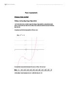
Change of sign method
Equation 3:
Since we are to compare the methods, we should use this method to find the root that was found in method 3, which lies between x=0 and x=1.
Use Autograph and Excel to find the required root, and we can see that it gives us the same value of 0.40303172 (correct to 8dp).
Newton-Raphson method
Equation 3:
We are required to find the same root which lies between x=0 and x=1.
It also finds the same value of the root which is corrected to 8dp successfully.
From the Excel tables of each method, we know that method 1 (change of sign method) takes 28 steps to find the root, while method 2 (Newton-Raphson method) and method 3 (rearrangement) take 4 and 17 steps respectively. In terms of speed of convergence, we can say that the Newton-Raphson method is the most efficient one.
However, if we compare them in terms of ease of use with available hardware and software, the change of sign method is the easiest one to use, since it involves least calculation. In change of sign method, we just need the original equation, however, in Newton-Raphson method, we need to calculate its derivative and in rearrangement method we need to rearrange the equation to get g(x). It can be illustrated more clearly in the following table.